Basic optimex Example
This notebook demonstrates the core optimex workflow using dummy processes — no external databases required.
We set up a simple system with two products, each producible via two alternative routes, and let optimex find the climate-optimal transition pathway.
The pipeline follows four steps:
- Database setup — biosphere, background, and foreground in Brightway
- LCA processing — extract time-explicit LCA data
- Optimization — find the cost-optimal deployment schedule
- Post-processing — visualize results
1. Database Setup
We create a standalone Brightway project with:
- A biosphere database (CO2, CH4, land occupation)
- Three background databases at different points in time (2020, 2035, 2050) representing evolving supply chains
- A foreground database with our decision-relevant processes
from datetime import datetime
import numpy as np
import bw2data as bd
from bw_temporalis import TemporalDistribution, easy_timedelta_distribution

bd.projects.set_current("optimex_basic_example")
Biosphere
Elementary flows that processes can emit or consume. When using ecoinvent, this is already available.
biosphere_data = {
    ("biosphere3", "CO2"): {
        "type": bd.labels.biosphere_node_default,
        "name": "carbon dioxide",
        "CAS number": "000124-38-9",
    },
    ("biosphere3", "CH4"): {
        "type": bd.labels.biosphere_node_default,
        "name": "methane, fossil",
        "CAS number": "000074-82-8",
    },
    ("biosphere3", "land_occupation"): {
        "type": bd.labels.biosphere_node_default,
        "name": "land occupation",
    },
}
bd.Database("biosphere3").write(biosphere_data)
100%|██████████| 3/3 [00:00<00:00, 12545.28it/s]

11:15:06+0100 [info     ] Vacuuming database
Characterization Methods
Maps elementary flows to impact scores. With ecoinvent, standard methods (IPCC, ReCiPe, ...) are pre-loaded.
bd.Method(("GWP", "example")).write(
    [
        (("biosphere3", "CO2"), 1),
        (("biosphere3", "CH4"), 27),
    ]
)

bd.Method(("land use", "example")).write(
    [
        (("biosphere3", "land_occupation"), 1),
        (("biosphere3", "CH4"), 27),
    ]
)
Background Databases
Background processes supply inputs to the foreground but are not decision variables. To model technological evolution, we provide multiple snapshots at different years. optimex interpolates between them.
Each database needs representative_time metadata so optimex knows which year it represents. In practice, tools like premise generate these from IAM scenarios.
# Background 2020
db_2020_data = {
    ("db_2020", "I1"): {
        "name": "node I1",
        "location": "somewhere",
        "type": bd.labels.chimaera_node_default,
        "reference product": "I1",
        "exchanges": [
            {
                "amount": 1,
                "type": bd.labels.production_edge_default,
                "input": ("db_2020", "I1"),
            },
            {
                "amount": 3000,
                "type": bd.labels.biosphere_edge_default,
                "input": ("biosphere3", "CO2"),
            },
        ],
    },
    ("db_2020", "I2"): {
        "name": "node I2",
        "location": "somewhere",
        "type": bd.labels.chimaera_node_default,
        "reference product": "I2",
        "exchanges": [
            {
                "amount": 1,
                "type": bd.labels.production_edge_default,
                "input": ("db_2020", "I2"),
            },
            {
                "amount": 5,
                "type": bd.labels.biosphere_edge_default,
                "input": ("biosphere3", "CH4"),
            },
        ],
    },
    ("db_2020", "I3"): {
        "name": "node I3",
        "location": "somewhere",
        "type": bd.labels.chimaera_node_default,
        "reference product": "I3",
        "exchanges": [
            {
                "amount": 1,
                "type": bd.labels.production_edge_default,
                "input": ("db_2020", "I3"),
            },
            {
                "amount": 3,
                "type": bd.labels.biosphere_edge_default,
                "input": ("biosphere3", "CH4"),
            },
            {
                "amount": 10,
                "type": bd.labels.biosphere_edge_default,
                "input": ("biosphere3", "land_occupation"),
            },
        ],
    },
}
bg_2020 = bd.Database("db_2020")
bg_2020.write(db_2020_data)
bg_2020.metadata["representative_time"] = datetime(2020, 1, 1).isoformat()
bg_2020.register()

# Background 2035 — lower emissions reflecting technological progress
db_2035_data = {
    ("db_2035", "I1"): {
        "name": "node I1",
        "location": "somewhere",
        "type": bd.labels.chimaera_node_default,
        "reference product": "I1",
        "exchanges": [
            {
                "amount": 1,
                "type": bd.labels.production_edge_default,
                "input": ("db_2035", "I1"),
            },
            {
                "amount": 2500,
                "type": bd.labels.biosphere_edge_default,
                "input": ("biosphere3", "CO2"),
            },
        ],
    },
    ("db_2035", "I2"): {
        "name": "node I2",
        "location": "somewhere",
        "type": bd.labels.chimaera_node_default,
        "reference product": "I2",
        "exchanges": [
            {
                "amount": 1,
                "type": bd.labels.production_edge_default,
                "input": ("db_2035", "I2"),
            },
            {
                "amount": 2,
                "type": bd.labels.biosphere_edge_default,
                "input": ("biosphere3", "CH4"),
            },
        ],
    },
    ("db_2035", "I3"): {
        "name": "node I3",
        "location": "somewhere",
        "type": bd.labels.chimaera_node_default,
        "reference product": "I3",
        "exchanges": [
            {
                "amount": 1,
                "type": bd.labels.production_edge_default,
                "input": ("db_2035", "I3"),
            },
            {
                "amount": 2,
                "type": bd.labels.biosphere_edge_default,
                "input": ("biosphere3", "CH4"),
            },
            {
                "amount": 7,
                "type": bd.labels.biosphere_edge_default,
                "input": ("biosphere3", "land_occupation"),
            },
        ],
    },
}
bg_2035 = bd.Database("db_2035")
bg_2035.write(db_2035_data)
bg_2035.metadata["representative_time"] = datetime(2035, 1, 1).isoformat()
bg_2035.register()

# Background 2050 — further improvements
db_2050_data = {
    ("db_2050", "I1"): {
        "name": "node I1",
        "location": "somewhere",
        "type": bd.labels.chimaera_node_default,
        "reference product": "I1",
        "exchanges": [
            {
                "amount": 1,
                "type": bd.labels.production_edge_default,
                "input": ("db_2050", "I1"),
            },
            {
                "amount": 2200,
                "type": bd.labels.biosphere_edge_default,
                "input": ("biosphere3", "CO2"),
            },
        ],
    },
    ("db_2050", "I2"): {
        "name": "node I2",
        "location": "somewhere",
        "type": bd.labels.chimaera_node_default,
        "reference product": "I2",
        "exchanges": [
            {
                "amount": 1,
                "type": bd.labels.production_edge_default,
                "input": ("db_2050", "I2"),
            },
            {
                "amount": 1,
                "type": bd.labels.biosphere_edge_default,
                "input": ("biosphere3", "CH4"),
            },
        ],
    },
    ("db_2050", "I3"): {
        "name": "node I3",
        "location": "somewhere",
        "type": bd.labels.chimaera_node_default,
        "reference product": "I3",
        "exchanges": [
            {
                "amount": 1,
                "type": bd.labels.production_edge_default,
                "input": ("db_2050", "I3"),
            },
            {
                "amount": 1,
                "type": bd.labels.biosphere_edge_default,
                "input": ("biosphere3", "CH4"),
            },
            {
                "amount": 7,
                "type": bd.labels.biosphere_edge_default,
                "input": ("biosphere3", "land_occupation"),
            },
        ],
    },
}
bg_2050 = bd.Database("db_2050")
bg_2050.write(db_2050_data)
bg_2050.metadata["representative_time"] = datetime(2050, 1, 1).isoformat()
bg_2050.register()
11:15:06+0100 [warning  ] Not able to determine geocollections for all datasets. This database is not ready for regionalization.


100%|██████████| 3/3 [00:00<00:00, 30393.51it/s]

11:15:06+0100 [info     ] Vacuuming database
11:15:06+0100 [warning  ] Not able to determine geocollections for all datasets. This database is not ready for regionalization.


100%|██████████| 3/3 [00:00<00:00, 58798.65it/s]

11:15:06+0100 [info     ] Vacuuming database
11:15:06+0100 [warning  ] Not able to determine geocollections for all datasets. This database is not ready for regionalization.


100%|██████████| 3/3 [00:00<00:00, 69518.85it/s]

11:15:06+0100 [info     ] Vacuuming database
Foreground Database
The foreground contains the decision-relevant processes whose installation and operation timing optimex optimizes.
Key optimex-specific attributes on processes and exchanges:
operation_time_limits: tuple(start, end)defining the operation phase within a process lifetimetemporal_distribution: when each exchange occurs relative to installation (usingTemporalDistribution)operation: True: marks exchanges that scale with operational level (production, operational emissions)
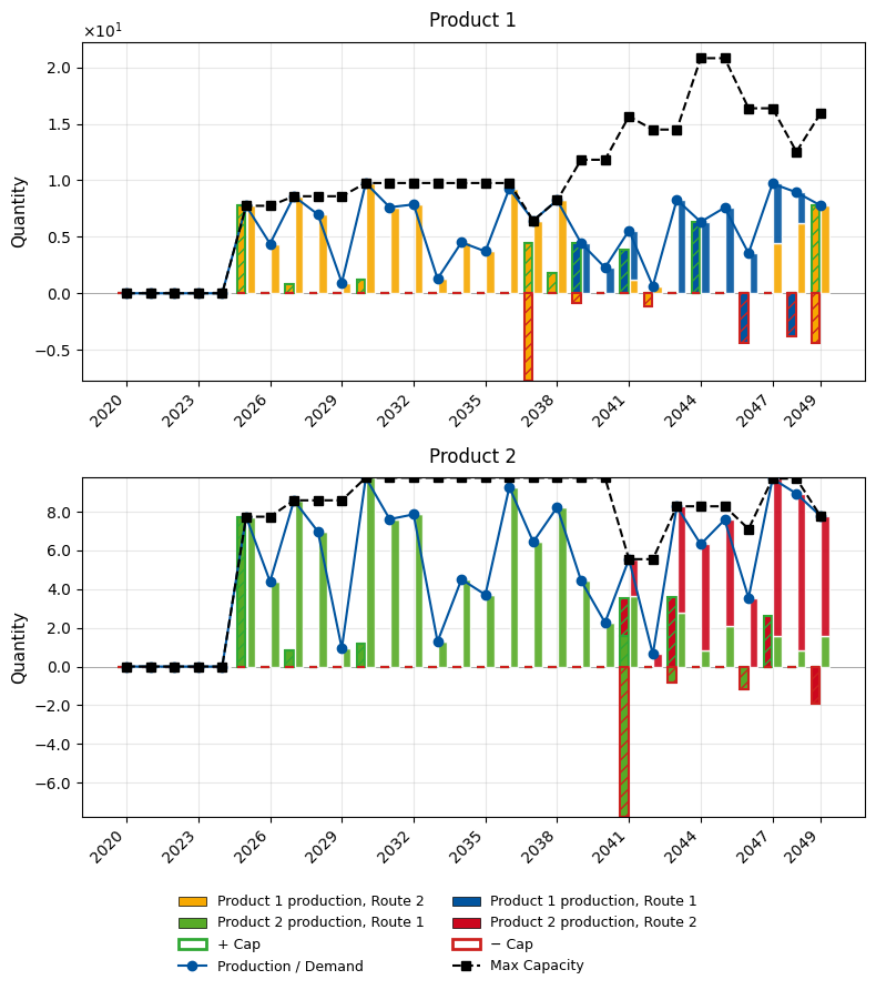
Our system has two products, each with two production routes:
- Product 1: Route 1 (6-year operation, uses I1+I3, captures CO2 during operation) vs. Route 2 (11-year operation, uses I2+I3, captures CO2 during operation)
- Product 2: Route 1 (15-year operation, needs Product 1, uses I3, emits CO2) vs. Route 2 (7-year operation, needs Product 1, uses I2, captures CO2 during operation)
if "foreground" in bd.databases:
    del bd.databases["foreground"]
foreground = bd.Database("foreground")
foreground.register()
foreground_data = {
    # --- Product 1 and its two production routes ---
    ("foreground", "Product 1"): {
        "name": "Product 1",
        "unit": "kg",
        "type": bd.labels.product_node_default,
    },
    ("foreground", "P1R1"): {
        "name": "Product 1 production, Route 1",
        "location": "somewhere",
        "type": bd.labels.process_node_default,
        "operation_time_limits": (0, 6),
        "exchanges": [
            {
                "amount": 1,
                "type": bd.labels.production_edge_default,
                "input": ("foreground", "Product 1"),
                "temporal_distribution": easy_timedelta_distribution(
                    start=1, end=6, steps=6, resolution="Y", kind="uniform"
                ),
                "operation": True,
            },
            {
                "amount": 27.5,
                "type": bd.labels.consumption_edge_default,
                "input": ("db_2020", "I1"),
                "temporal_distribution": TemporalDistribution(
                    date=np.array([11], dtype="timedelta64[Y]"), amount=np.array([1])
                ),
            },
            {
                "amount": 35,
                "type": bd.labels.consumption_edge_default,
                "input": ("db_2020", "I3"),
                "temporal_distribution": TemporalDistribution(
                    date=np.array([11], dtype="timedelta64[Y]"), amount=np.array([1])
                ),
            },
            {
                "amount": -20,
                "type": bd.labels.biosphere_edge_default,
                "input": ("biosphere3", "CO2"),
                "temporal_distribution": easy_timedelta_distribution(
                    start=1, end=6, steps=6, resolution="Y", kind="uniform"
                ),
                "operation": True,
            },
        ],
    },
    ("foreground", "P1R2"): {
        "name": "Product 1 production, Route 2",
        "location": "somewhere",
        "type": bd.labels.process_node_default,
        "operation_time_limits": (0, 11),
        "exchanges": [
            {
                "amount": 1,
                "type": bd.labels.production_edge_default,
                "input": ("foreground", "Product 1"),
                "temporal_distribution": easy_timedelta_distribution(
                    start=1, end=11, steps=11, resolution="Y", kind="uniform"
                ),
                "operation": True,
            },
            {
                "amount": 10,
                "type": bd.labels.consumption_edge_default,
                "input": ("db_2020", "I2"),
                "temporal_distribution": TemporalDistribution(
                    date=np.array([11], dtype="timedelta64[Y]"), amount=np.array([1])
                ),
            },
            {
                "amount": 5,
                "type": bd.labels.consumption_edge_default,
                "input": ("db_2020", "I3"),
                "temporal_distribution": TemporalDistribution(
                    date=np.array([11], dtype="timedelta64[Y]"), amount=np.array([1])
                ),
            },
            {
                "amount": -20,
                "type": bd.labels.biosphere_edge_default,
                "input": ("biosphere3", "CO2"),
                "temporal_distribution": easy_timedelta_distribution(
                    start=1, end=11, steps=11, resolution="Y", kind="uniform"
                ),
                "operation": True,
            },
        ],
    },
    # --- Product 2 and its two production routes ---
    ("foreground", "Product 2"): {
        "name": "Product 2",
        "unit": "kg",
        "type": bd.labels.product_node_default,
    },
    ("foreground", "P2R1"): {
        "name": "Product 2 production, Route 1",
        "location": "somewhere",
        "type": bd.labels.process_node_default,
        "operation_time_limits": (0, 15),
        "exchanges": [
            {
                "amount": 1,
                "type": bd.labels.production_edge_default,
                "input": ("foreground", "Product 2"),
                "temporal_distribution": easy_timedelta_distribution(
                    start=1, end=15, steps=15, resolution="Y", kind="uniform"
                ),
                "operation": True,
            },
            {
                "amount": 1,
                "type": bd.labels.consumption_edge_default,
                "input": ("foreground", "Product 1"),
                "temporal_distribution": easy_timedelta_distribution(
                    start=1, end=15, steps=15, resolution="Y", kind="uniform"
                ),
                "operation": True,
            },
            {
                "amount": 18.5,
                "type": bd.labels.consumption_edge_default,
                "input": ("db_2020", "I3"),
                "temporal_distribution": TemporalDistribution(
                    date=np.array([0], dtype="timedelta64[Y]"), amount=np.array([1])
                ),
            },
            {
                "amount": 3,
                "type": bd.labels.biosphere_edge_default,
                "input": ("biosphere3", "CO2"),
                "temporal_distribution": easy_timedelta_distribution(
                    start=1, end=15, steps=15, resolution="Y", kind="uniform"
                ),
                "operation": True,
            },
        ],
    },
    ("foreground", "P2R2"): {
        "name": "Product 2 production, Route 2",
        "location": "somewhere",
        "type": bd.labels.process_node_default,
        "operation_time_limits": (0, 7),
        "exchanges": [
            {
                "amount": 1,
                "type": bd.labels.production_edge_default,
                "input": ("foreground", "Product 2"),
                "temporal_distribution": easy_timedelta_distribution(
                    start=1, end=7, steps=7, resolution="Y", kind="uniform"
                ),
                "operation": True,
            },
            {
                "amount": 1,
                "type": bd.labels.consumption_edge_default,
                "input": ("foreground", "Product 1"),
                "temporal_distribution": easy_timedelta_distribution(
                    start=1, end=7, steps=7, resolution="Y", kind="uniform"
                ),
                "operation": True,
            },
            {
                "amount": 15.5,
                "type": bd.labels.consumption_edge_default,
                "input": ("db_2020", "I2"),
                "temporal_distribution": TemporalDistribution(
                    date=np.array([0], dtype="timedelta64[Y]"), amount=np.array([1])
                ),
            },
            {
                "amount": -10,
                "type": bd.labels.biosphere_edge_default,
                "input": ("biosphere3", "CO2"),
                "temporal_distribution": easy_timedelta_distribution(
                    start=1, end=7, steps=7, resolution="Y", kind="uniform"
                ),
                "operation": True,
            },
        ],
    },
}

fg = bd.Database("foreground")
fg.write(foreground_data)
fg.register()
11:15:06+0100 [warning  ] Not able to determine geocollections for all datasets. This database is not ready for regionalization.


100%|██████████| 6/6 [00:00<00:00, 21041.66it/s]

11:15:06+0100 [info     ] Vacuuming database
Demand
Define time-varying demand for Product 2 from 2025 to 2049. optimex will determine the optimal process mix to meet this demand each year.
years = range(2025, 2050)
rng = np.random.default_rng(42)

td_demand = TemporalDistribution(
    date=np.array(
        [datetime(year, 1, 1).isoformat() for year in years], dtype="datetime64[s]"
    ),
    amount=rng.random(len(years)) * 10,
)

functional_demand = {bd.get_node(database="foreground", name="Product 2"): td_demand}
2. LCA Processing
Configure the LCA: specify the demand, temporal settings, and characterization methods. The LCADataProcessor extracts all time-explicit LCA tensors needed for optimization.
from optimex import lca_processor
lca_config = lca_processor.LCAConfig(
demand=functional_demand,
temporal={
"start_date": datetime(2020, 1, 1),
"temporal_resolution": "year",
"time_horizon": 100,
},
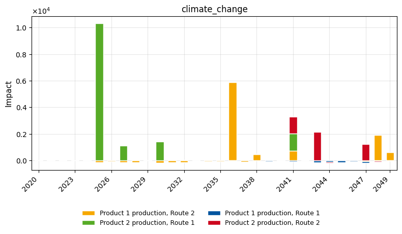
characterization_methods=[
{
"category_name": "climate_change",
"brightway_method": ("GWP", "example"),
},
],
)
lca_data_processor = lca_processor.LCADataProcessor(lca_config)
2026-02-11 11:15:06.146 | INFO     | optimex.lca_processor:_parse_demand:417 - Identified demand in system time range of %s for products %s
2026-02-11 11:15:06.150 | INFO     | optimex.lca_processor:_construct_foreground_tensors:639 - Constructed foreground tensors.
2026-02-11 11:15:06.151 | INFO     | optimex.lca_processor:log_tensor_dimensions:634 - Technosphere (external) shape: (4 processes, 3 flows, 2 years) with 6 total entries.
2026-02-11 11:15:06.151 | INFO     | optimex.lca_processor:log_tensor_dimensions:634 - Internal demand shape: (2 processes, 1 flows, 15 years) with 22 total entries.
2026-02-11 11:15:06.151 | INFO     | optimex.lca_processor:log_tensor_dimensions:634 - Biosphere shape: (4 processes, 1 flows, 15 years) with 39 total entries.
2026-02-11 11:15:06.151 | INFO     | optimex.lca_processor:log_tensor_dimensions:634 - Production shape: (4 processes, 2 flows, 15 years) with 39 total entries.
2026-02-11 11:15:06.152 | INFO     | optimex.lca_processor:_calculate_inventory_of_db:678 - Calculating inventory for database: db_2020
2026-02-11 11:15:06.158 | INFO     | optimex.lca_processor:_calculate_inventory_of_db:694 - Factorized LCI for database: db_2020
100%|██████████| 3/3 [00:00<00:00, 223.28it/s]
2026-02-11 11:15:06.173 | INFO     | optimex.lca_processor:_calculate_inventory_of_db:734 - Finished calculating inventory for database: db_2020
2026-02-11 11:15:06.173 | INFO     | optimex.lca_processor:_calculate_inventory_of_db:678 - Calculating inventory for database: db_2035
2026-02-11 11:15:06.178 | INFO     | optimex.lca_processor:_calculate_inventory_of_db:694 - Factorized LCI for database: db_2035
100%|██████████| 3/3 [00:00<00:00, 277.65it/s]
2026-02-11 11:15:06.189 | INFO     | optimex.lca_processor:_calculate_inventory_of_db:734 - Finished calculating inventory for database: db_2035
2026-02-11 11:15:06.190 | INFO     | optimex.lca_processor:_calculate_inventory_of_db:678 - Calculating inventory for database: db_2050
2026-02-11 11:15:06.194 | INFO     | optimex.lca_processor:_calculate_inventory_of_db:694 - Factorized LCI for database: db_2050
100%|██████████| 3/3 [00:00<00:00, 261.19it/s]
2026-02-11 11:15:06.207 | INFO     | optimex.lca_processor:_calculate_inventory_of_db:734 - Finished calculating inventory for database: db_2050
2026-02-11 11:15:06.207 | INFO     | optimex.lca_processor:_prepare_background_inventory:841 - Computed background inventory using method: sequential
2026-02-11 11:15:06.209 | INFO     | optimex.lca_processor:_construct_characterization_tensor:952 - Static characterization for method climate_change completed.
2026-02-11 11:15:06.210 | INFO     | optimex.lca_processor:_construct_mapping_matrix:895 - Constructed mapping matrix for background databases based on linear interpolation.
Convert to Optimization Inputs
The ModelInputManager converts LCA data into OptimizationModelInputs. These can be saved/loaded to avoid re-running the LCA step.
from optimex import converter

manager = converter.ModelInputManager()
optimization_model_inputs = manager.parse_from_lca_processor(lca_data_processor)

# Optionally save/load:
# manager.save("model_inputs.json")
# manager.load_inputs("model_inputs.json")
3. Optimization
Create and solve the optimization model. The objective is to minimize total climate change impact over the system time horizon.
from optimex import optimizer

model = optimizer.create_model(
    optimization_model_inputs,
    name="basic_example",
    objective_category="climate_change",
)
2026-02-11 11:15:06.421 | INFO     | optimex.optimizer:create_model:116 - Creating sets
2026-02-11 11:15:06.422 | INFO     | optimex.optimizer:create_model:158 - Creating parameters
2026-02-11 11:15:06.423 | INFO     | optimex.optimizer:create_model:448 - Creating variables
2026-02-11 11:15:06.919 | INFO     | optimex.optimizer:solve_model:1113 - Solver [glpk] termination: optimal
2026-02-11 11:15:06.936 | INFO     | optimex.optimizer:solve_model:1127 - Objective (scaled): 27.3871
2026-02-11 11:15:06.936 | INFO     | optimex.optimizer:solve_model:1128 - Objective (real):   25880.8
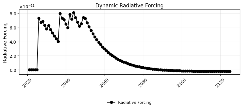
4. Post-processing
Visualize the optimal transition pathway: installations, operations, production vs. demand, and environmental impacts.
from optimex import postprocessing

pp = postprocessing.PostProcessor(m, plot_config={"figsize": (8, 4)})
pp.plot_characterized_dynamic_inventory(
    base_lcia_method=("GWP", "example"), biosphere_database="biosphere3"
)
2026-02-11 11:15:07.822 | INFO | dynamic_characterization.dynamic_characterization:characterize:82 - No custom dynamic characterization functions provided. Using default dynamic characterization functions. The flows that are characterized are based on the selection of the initially chosen impact category.