Methanol & Pig Iron Case Study
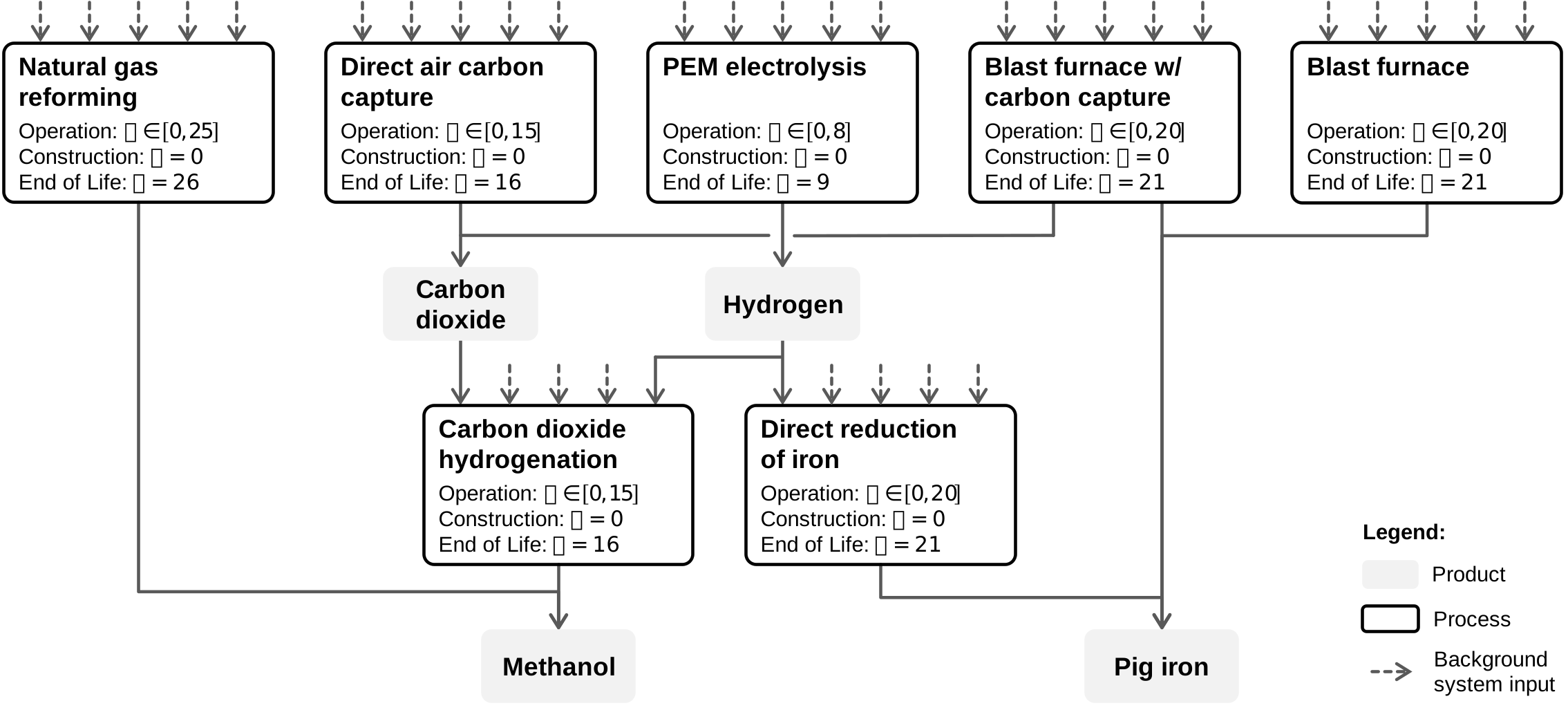
This notebook demonstrates optimex on a realistic case study using ecoinvent and premise (REMIND-EU SSP2-NDC scenario) databases. It optimizes the transition pathway for two coupled product systems:
- Methanol: via CO2 hydrogenation (green route) or natural gas reforming (conventional)
- Pig iron: via H2-based direct reduction, blast furnace with carbon capture, or conventional blast furnace
Intermediate products (hydrogen, captured CO2) create cross-linkages between the systems.
Prerequisites: ecoinvent 3.12 + premise databases must be set up (see premise_database_setup.ipynb).
/Users/timodiepers/Documents/Coding/optimex/.venv/lib/python3.13/site-packages/bw2calc/__init__.py:53: UserWarning:
It seems like you have an ARM architecture, but haven't installed scikit-umfpack:

    https://pypi.org/project/scikit-umfpack/

Installing it could give you much faster calculations.

  warnings.warn(UMFPACK_WARNING)
Background Inputs from ecoinvent/premise
Retrieve background processes (electricity, heat, water, infrastructure, raw materials) and biosphere flows from the premise-modified ecoinvent databases.
electricity_mv = bd.get_node(
    database="ei312_REMIND-EU_SSP2_NDC_2020",
    name="market group for electricity, medium voltage",
    location="RER",
)
electricity_lv = bd.get_node(
    database="ei312_REMIND-EU_SSP2_NDC_2020",
    name="market group for electricity, low voltage",
    location="RER",
)
heat = bd.get_node(
    database="ei312_REMIND-EU_SSP2_NDC_2020",
    name="market for heat, district or industrial",
    location="DEU",
)  # Process not available for RER
water_tap = bd.get_node(
    database="ei312_REMIND-EU_SSP2_NDC_2020",
    name="market for tap water",
    location="Europe without Switzerland",
)
water_deionized = bd.get_node(
    database="ei312_REMIND-EU_SSP2_NDC_2020",
    name="deionized water production, via reverse osmosis, from brackish water",
    location="RER",
)

dac_system = bd.get_node(
    database="ei312_REMIND-EU_SSP2_NDC_2020",
    name="direct air capture system, solvent-based, 1MtCO2",
    location="RER",
)
dac_system_eol = bd.get_node(
    database="ei312_REMIND-EU_SSP2_NDC_2020",
    name="treatment of direct air capture system, solvent-based, 1MtCO2",
    location="RER",
)

pem_stack = bd.get_node(
    database="ei312_REMIND-EU_SSP2_NDC_2020",
    name="electrolyzer production, 1MWe, PEM, Stack",
    location="RER",
)
pem_stack_eol = bd.get_node(
    database="ei312_REMIND-EU_SSP2_NDC_2020",
    name="treatment of electrolyzer stack, 1MWe, PEM",
    location="RER",
)
pem_bop = bd.get_node(
    database="ei312_REMIND-EU_SSP2_NDC_2020",
    name="electrolyzer production, 1MWe, PEM, Balance of Plant",
    location="RER",
)
pem_bop_eol = bd.get_node(
    database="ei312_REMIND-EU_SSP2_NDC_2020",
    name="treatment of electrolyzer balance of plant, 1MWe, PEM",
    location="RER",
)

methanol_production_facility = bd.get_node(
    database="ei312_REMIND-EU_SSP2_NDC_2020",
    name="methanol production facility, construction",
    location="RER",
)

blast_furnace_production = bd.get_node(
    database="ei312_REMIND-EU_SSP2_NDC_2020",
    name="market for blast furnace",
    location="GLO",
)
coke = bd.get_node(
    database="ei312_REMIND-EU_SSP2_NDC_2020", name="market for coke", location="RoW"
)
hard_coal = bd.get_node(
    database="ei312_REMIND-EU_SSP2_NDC_2020",
    name="market group for hard coal",
    location="RER",
)
iron_ore_concentrate = bd.get_node(
    database="ei312_REMIND-EU_SSP2_NDC_2020",
    name="market for iron ore concentrate",
    location="World",
)
iron_sinter = bd.get_node(
    database="ei312_REMIND-EU_SSP2_NDC_2020",
    name="iron sinter production",
    location="RER",
)
iron_pellet = bd.get_node(
    database="ei312_REMIND-EU_SSP2_NDC_2020",
    name="market for iron pellet",
    location="GLO",
)
natural_gas = bd.get_node(
    database="ei312_REMIND-EU_SSP2_NDC_2020",
    name="petroleum and gas production, offshore",
    product="natural gas, high pressure",
    location="DE",
)

methanol_factory_ng = bd.get_node(
    database="ei312_REMIND-EU_SSP2_NDC_2020",
    name="market for methanol factory",
    location="GLO",
)
co2 = bd.get_node(
    database="ecoinvent-3.12-biosphere",
    name="Carbon dioxide, fossil",
    categories=("air",),
)

particulate_matter_sm = bd.get_node(
    database="ecoinvent-3.12-biosphere",
    name="Particulate Matter, < 2.5 um",
    categories=("air",),
)
particulate_matter_md = bd.get_node(
    database="ecoinvent-3.12-biosphere",
    name="Particulate Matter, > 2.5 um and < 10um",
    categories=("air",),
)
particulate_matter_lg = bd.get_node(
    database="ecoinvent-3.12-biosphere",
    name="Particulate Matter, > 10 um",
    categories=("air",),
)
Foreground Setup
Define the decision-relevant foreground system. Each process has:
operation_time_limits: when the operation phase occurs within the process lifetimeoperation=Trueon exchanges that scale with operational levelvintage_improvements: efficiency gains for processes installed in later years- Construction and end-of-life exchanges with appropriate temporal distributions
Helper functions (infer_operation_td_from_limits, etc.) automatically generate temporal distributions from the operation time limits.
if "foreground" in bd.databases:
    del bd.databases["foreground"]  # to make sure we create the foreground from scratch
foreground = bd.Database("foreground")
foreground.register()
Products
Four products in the system: methanol and pig iron (final demand), hydrogen and captured CO2 (intermediates).
methanol = foreground.new_node(
    name="methanol",
    code="methanol",
    unit="kg",
    type=bd.labels.product_node_default,
)
methanol.save()

iron = foreground.new_node(
    name="pig iron",
    code="pig iron",
    unit="kg",
    type=bd.labels.product_node_default,
)
iron.save()

hydrogen = foreground.new_node(
    name="hydrogen",
    code="hydrogen",
    unit="kg",
    type=bd.labels.product_node_default,
)
hydrogen.save()

captured_co2 = foreground.new_node(
    name="captured CO2",
    code="captured CO2",
    unit="kg",
    type=bd.labels.product_node_default,
)
captured_co2.save()
Processes
from optimex.utils import (
    infer_operation_td_from_limits,
    infer_construction_td_from_limits,
    infer_eol_td_from_limits,
)
Direct Air Capture (DAC)
Solvent-based DAC producing captured CO2. 15-year operation lifetime. Electricity and heat consumption improve with vintage year.
dac = foreground.new_node(
    name="direct air carbon capture",
    code="direct air carbon capture",
    location="RER",
    type=bd.labels.process_node_default,
    operation_time_limits=(0, 15),
)
dac.save()
# operation
dac.new_edge(
    input=captured_co2,
    amount=1.0,
    type=bd.labels.production_edge_default,
    operation=True,
    temporal_distribution=infer_operation_td_from_limits(dac),
).save()

dac.new_edge(
    input=electricity_mv,
    amount=0.345,
    type=bd.labels.consumption_edge_default,
    operation=True,
    temporal_distribution=infer_operation_td_from_limits(dac),
).save()

dac.new_edge(
    input=heat,
    amount=6.28,
    type=bd.labels.consumption_edge_default,
    operation=True,
    temporal_distribution=infer_operation_td_from_limits(dac),
).save()

dac.new_edge(
    input=water_tap,
    amount=3.437,
    type=bd.labels.consumption_edge_default,
    operation=True,
    temporal_distribution=infer_operation_td_from_limits(dac),
).save()

dac.new_edge(
    input=co2,
    amount=-1.0,
    type=bd.labels.biosphere_edge_default,
    operation=True,
    temporal_distribution=infer_operation_td_from_limits(dac),
).save()

# construction
dac.new_edge(
    input=dac_system,
    amount=5e-11,  # 5e-11
    type=bd.labels.consumption_edge_default,
    temporal_distribution=infer_construction_td_from_limits(dac),
).save()

# end-of-life
dac.new_edge(
    input=dac_system_eol,
    amount=-5e-11,  # 5e-11
    type=bd.labels.consumption_edge_default,
    temporal_distribution=infer_eol_td_from_limits(dac),
).save()
PEM Electrolysis
Produces hydrogen from electricity and water. 8-year stack lifetime. Electricity consumption improves with vintage.
pem = foreground.new_node(
    name="PEM Electrolysis",
    code="PEM Electrolysis",
    location="RER",
    type=bd.labels.process_node_default,
    operation_time_limits=(0, 8),
)
pem.save()
# operation
pem.new_edge(
    input=hydrogen,
    amount=1.0,
    type=bd.labels.production_edge_default,
    operation=True,
    temporal_distribution=infer_operation_td_from_limits(pem),
).save()

pem.new_edge(
    input=electricity_lv,
    amount=54,
    type=bd.labels.consumption_edge_default,
    operation=True,
    temporal_distribution=infer_operation_td_from_limits(pem),
).save()

pem.new_edge(
    input=water_deionized,
    amount=14,
    type=bd.labels.consumption_edge_default,
    operation=True,
    temporal_distribution=infer_operation_td_from_limits(pem),
).save()

# construction
pem.new_edge(
    input=pem_stack,
    amount=1.34989e-6,
    type=bd.labels.consumption_edge_default,
    temporal_distribution=infer_construction_td_from_limits(pem),
).save()

pem.new_edge(
    input=pem_bop,
    amount=3.37373e-7,
    type=bd.labels.consumption_edge_default,
    temporal_distribution=infer_construction_td_from_limits(pem),
).save()

# end-of-life
pem.new_edge(
    input=pem_stack_eol,
    amount=-1.34989e-6,
    type=bd.labels.consumption_edge_default,
    temporal_distribution=infer_eol_td_from_limits(pem),
).save()

pem.new_edge(
    input=pem_bop_eol,
    amount=-3.37373e-7,
    type=bd.labels.consumption_edge_default,
    temporal_distribution=infer_eol_td_from_limits(pem),
).save()
CO2 Hydrogenation to Methanol
Green methanol route: combines hydrogen and captured CO2. 15-year lifetime. Electricity consumption and CO2 emissions improve with vintage.
co2_hydrogenation = foreground.new_node(
    name="Carbon dioxide hydrogenation to methanol",
    code="Carbon dioxide hydrogenation to methanol",
    location="RER",
    type=bd.labels.process_node_default,
    operation_time_limits=(0, 15),
)
co2_hydrogenation.save()
# operation
co2_hydrogenation.new_edge(
    input=methanol,
    amount=1.0,
    type=bd.labels.production_edge_default,
    operation=True,
    temporal_distribution=infer_operation_td_from_limits(co2_hydrogenation),
).save()

co2_hydrogenation.new_edge(
    input=hydrogen,
    amount=0.138975,
    type=bd.labels.consumption_edge_default,
    operation=True,
    temporal_distribution=infer_operation_td_from_limits(co2_hydrogenation),
).save()

co2_hydrogenation.new_edge(
    input=captured_co2,
    amount=1.690523,
    type=bd.labels.consumption_edge_default,
    operation=True,
    temporal_distribution=infer_operation_td_from_limits(co2_hydrogenation),
).save()

co2_hydrogenation.new_edge(
    input=electricity_lv,
    amount=0.302895,
    type=bd.labels.consumption_edge_default,
    operation=True,
    temporal_distribution=infer_operation_td_from_limits(co2_hydrogenation),
).save()

co2_hydrogenation.new_edge(
    input=water_tap,
    amount=0.81959,
    type=bd.labels.consumption_edge_default,
    operation=True,
    temporal_distribution=infer_operation_td_from_limits(co2_hydrogenation),
).save()

co2_hydrogenation.new_edge(
    input=co2,
    amount=0.32,
    type=bd.labels.biosphere_edge_default,
    operation=True,
    temporal_distribution=infer_operation_td_from_limits(co2_hydrogenation),
).save()

# construction
co2_hydrogenation.new_edge(
    input=methanol_production_facility,
    amount=12.89,
    type=bd.labels.consumption_edge_default,
    temporal_distribution=infer_construction_td_from_limits(co2_hydrogenation),
).save()
Blast Furnace with Carbon Capture
Conventional iron production with post-combustion CO2 capture. Co-produces pig iron and captured CO2. 25-year lifetime. PM emissions reduced by 50% through co-capture.
blast_furnace_cc = foreground.new_node(
    name="Blast furnace with carbon capture",
    code="Blast furnace with carbon capture",
    location="RER",
    type=bd.labels.process_node_default,
    operation_time_limits=(0, 25),
)
blast_furnace_cc.save()
total_co2_emission_per_kg_iron = 0.849
captured_co2_per_kg_iron = 0.7054  # Happrecht et al., 2025, SI Section 1.3.2
total_pm_sm_emission_per_kg_iron = 2.8723e-5
total_pm_md_emission_per_kg_iron = 1.5957e-6
total_pm_lg_emission_per_kg_iron = 1.5957e-6
pm_emission_reduction = (
    0.5  # PM reduction through co-capture, Choi, 2013; Singh et al., 2011
)

# operation
blast_furnace_cc.new_edge(
    input=iron,
    amount=1.0,
    type=bd.labels.production_edge_default,
    operation=True,
    temporal_distribution=infer_operation_td_from_limits(blast_furnace_cc),
).save()

blast_furnace_cc.new_edge(
    input=captured_co2,
    amount=captured_co2_per_kg_iron,
    type=bd.labels.production_edge_default,
    operation=True,
    temporal_distribution=infer_operation_td_from_limits(blast_furnace_cc),
).save()

blast_furnace_cc.new_edge(
    input=co2,
    amount=total_co2_emission_per_kg_iron - captured_co2_per_kg_iron,
    type=bd.labels.biosphere_edge_default,
    operation=True,
    temporal_distribution=infer_operation_td_from_limits(blast_furnace_cc),
).save()

blast_furnace_cc.new_edge(
    input=natural_gas,
    amount=2.71 / 36,  # Happrecht et al., 2025, SI Section 1.3.2 w/ 36 MJ/m3
    type=bd.labels.consumption_edge_default,
    operation=True,
    temporal_distribution=infer_operation_td_from_limits(blast_furnace_cc),
).save()

blast_furnace_cc.new_edge(
    input=coke,
    amount=9.724,
    type=bd.labels.consumption_edge_default,
    operation=True,
    temporal_distribution=infer_operation_td_from_limits(blast_furnace_cc),
).save()

blast_furnace_cc.new_edge(
    input=hard_coal,
    amount=0.15,
    type=bd.labels.consumption_edge_default,
    operation=True,
    temporal_distribution=infer_operation_td_from_limits(blast_furnace_cc),
).save()

blast_furnace_cc.new_edge(
    input=iron_ore_concentrate,
    amount=0.15,
    type=bd.labels.consumption_edge_default,
    operation=True,
    temporal_distribution=infer_operation_td_from_limits(blast_furnace_cc),
).save()

blast_furnace_cc.new_edge(
    input=iron_pellet,
    amount=0.4,
    type=bd.labels.consumption_edge_default,
    operation=True,
    temporal_distribution=infer_operation_td_from_limits(blast_furnace_cc),
).save()

blast_furnace_cc.new_edge(
    input=iron_sinter,
    amount=1.05,
    type=bd.labels.consumption_edge_default,
    operation=True,
    temporal_distribution=infer_operation_td_from_limits(blast_furnace_cc),
).save()

blast_furnace_cc.new_edge(
    input=particulate_matter_sm,
    amount=(1 - pm_emission_reduction) * total_pm_sm_emission_per_kg_iron,
    type=bd.labels.biosphere_edge_default,
    operation=True,
    temporal_distribution=infer_operation_td_from_limits(blast_furnace_cc),
).save()

blast_furnace_cc.new_edge(
    input=particulate_matter_md,
    amount=(1 - pm_emission_reduction) * total_pm_md_emission_per_kg_iron,
    type=bd.labels.biosphere_edge_default,
    operation=True,
    temporal_distribution=infer_operation_td_from_limits(blast_furnace_cc),
).save()

blast_furnace_cc.new_edge(
    input=particulate_matter_lg,
    amount=(1 - pm_emission_reduction) * total_pm_lg_emission_per_kg_iron,
    type=bd.labels.biosphere_edge_default,
    operation=True,
    temporal_distribution=infer_operation_td_from_limits(blast_furnace_cc),
).save()

# construction
blast_furnace_cc.new_edge(
    input=blast_furnace_production,
    amount=1.333e-11,
    type=bd.labels.consumption_edge_default,
    temporal_distribution=infer_construction_td_from_limits(blast_furnace_cc),
).save()
Blast Furnace (conventional)
Standard blast furnace without carbon capture. Same inputs as above but full CO2 and PM emissions. 25-year lifetime.
blast_furnace = foreground.new_node(
    name="Blast furnace",
    code="Blast furnace",
    location="RER",
    type=bd.labels.process_node_default,
    operation_time_limits=(0, 25),
)
blast_furnace.save()
# operation
blast_furnace.new_edge(
    input=iron,
    amount=1.0,
    type=bd.labels.production_edge_default,
    operation=True,
    temporal_distribution=infer_operation_td_from_limits(blast_furnace),
).save()

blast_furnace.new_edge(
    input=co2,
    amount=total_co2_emission_per_kg_iron,
    type=bd.labels.biosphere_edge_default,
    operation=True,
    temporal_distribution=infer_operation_td_from_limits(blast_furnace),
).save()

blast_furnace.new_edge(
    input=natural_gas,
    amount=2.71 / 36,  # Happrecht et al., 2025, SI Section 1.3.2 w/ 36 MJ/m3
    type=bd.labels.consumption_edge_default,
    operation=True,
    temporal_distribution=infer_operation_td_from_limits(blast_furnace),
).save()

blast_furnace.new_edge(
    input=coke,
    amount=9.724,
    type=bd.labels.consumption_edge_default,
    operation=True,
    temporal_distribution=infer_operation_td_from_limits(blast_furnace),
).save()

blast_furnace.new_edge(
    input=hard_coal,
    amount=0.15,
    type=bd.labels.consumption_edge_default,
    operation=True,
    temporal_distribution=infer_operation_td_from_limits(blast_furnace),
).save()

blast_furnace.new_edge(
    input=iron_ore_concentrate,
    amount=0.15,
    type=bd.labels.consumption_edge_default,
    operation=True,
    temporal_distribution=infer_operation_td_from_limits(blast_furnace),
).save()

blast_furnace.new_edge(
    input=iron_pellet,
    amount=0.4,
    type=bd.labels.consumption_edge_default,
    operation=True,
    temporal_distribution=infer_operation_td_from_limits(blast_furnace),
).save()

blast_furnace.new_edge(
    input=iron_sinter,
    amount=1.05,
    type=bd.labels.consumption_edge_default,
    operation=True,
    temporal_distribution=infer_operation_td_from_limits(blast_furnace),
).save()

blast_furnace.new_edge(
    input=particulate_matter_sm,
    amount=total_pm_sm_emission_per_kg_iron,
    type=bd.labels.biosphere_edge_default,
    operation=True,
    temporal_distribution=infer_operation_td_from_limits(blast_furnace),
).save()

blast_furnace.new_edge(
    input=particulate_matter_md,
    amount=total_pm_md_emission_per_kg_iron,
    type=bd.labels.biosphere_edge_default,
    operation=True,
    temporal_distribution=infer_operation_td_from_limits(blast_furnace),
).save()

blast_furnace.new_edge(
    input=particulate_matter_lg,
    amount=total_pm_lg_emission_per_kg_iron,
    type=bd.labels.biosphere_edge_default,
    operation=True,
    temporal_distribution=infer_operation_td_from_limits(blast_furnace),
).save()

# construction
blast_furnace.new_edge(
    input=blast_furnace_production,
    amount=1.333e-11,
    type=bd.labels.consumption_edge_default,
    temporal_distribution=infer_construction_td_from_limits(blast_furnace),
).save()
Direct Reduction of Iron (H2-DRI)
Hydrogen-based iron reduction with much lower direct CO2 emissions. Consumes hydrogen, iron pellets, natural gas, and electricity. 25-year lifetime.
direct_reduction = foreground.new_node(
    name="Direct reduction of iron",
    code="Direct reduction of iron",
    location="RER",
    type=bd.labels.process_node_default,
    operation_time_limits=(0, 25),
)
direct_reduction.save()
dri_h2_consumption = 0.06264
dri_iron_pellet_consumption = 1.359733

# operation
direct_reduction.new_edge(
    input=iron,
    amount=1.0,
    type=bd.labels.production_edge_default,
    operation=True,
    temporal_distribution=infer_operation_td_from_limits(direct_reduction),
).save()

direct_reduction.new_edge(
    input=co2,
    amount=0.03271,
    type=bd.labels.biosphere_edge_default,
    operation=True,
    temporal_distribution=infer_operation_td_from_limits(direct_reduction),
).save()

direct_reduction.new_edge(
    input=hydrogen,
    amount=dri_h2_consumption,
    type=bd.labels.consumption_edge_default,
    operation=True,
    temporal_distribution=infer_operation_td_from_limits(direct_reduction),
).save()

direct_reduction.new_edge(
    input=natural_gas,
    amount=0.0358938,
    type=bd.labels.consumption_edge_default,
    operation=True,
    temporal_distribution=infer_operation_td_from_limits(direct_reduction),
).save()

direct_reduction.new_edge(
    input=iron_pellet,
    amount=dri_iron_pellet_consumption,
    type=bd.labels.consumption_edge_default,
    operation=True,
    temporal_distribution=infer_operation_td_from_limits(direct_reduction),
).save()

direct_reduction.new_edge(
    input=electricity_mv,
    amount=0.0192446
    + dri_h2_consumption * 4.024497
    + dri_iron_pellet_consumption * 0.27267,  # incl. h2 and iron pellet preheating
    type=bd.labels.consumption_edge_default,
    operation=True,
    temporal_distribution=infer_operation_td_from_limits(direct_reduction),
).save()

# construction
direct_reduction.new_edge(
    input=blast_furnace_production,
    amount=1.333e-11,
    type=bd.labels.consumption_edge_default,
    temporal_distribution=infer_construction_td_from_limits(direct_reduction),
).save()
Natural Gas Reforming to Methanol
Conventional methanol production from natural gas. 25-year lifetime. No vintage improvements.
ng_reforming = foreground.new_node(
    name="Natural gas reforming",
    code="Natural gas reforming",
    location="RER",
    type=bd.labels.process_node_default,
    operation_time_limits=(0, 25),
)
ng_reforming.save()
# operation
ng_reforming.new_edge(
    input=methanol,
    amount=1.0,
    type=bd.labels.production_edge_default,
    operation=True,
    temporal_distribution=infer_operation_td_from_limits(ng_reforming),
).save()

ng_reforming.new_edge(
    input=co2,
    amount=0.33424,
    type=bd.labels.biosphere_edge_default,
    operation=True,
    temporal_distribution=infer_operation_td_from_limits(ng_reforming),
).save()


ng_reforming.new_edge(
    input=natural_gas,
    amount=0.8895,
    type=bd.labels.consumption_edge_default,
    operation=True,
    temporal_distribution=infer_operation_td_from_limits(ng_reforming),
).save()

ng_reforming.new_edge(
    input=water_deionized,
    amount=0.355,
    type=bd.labels.consumption_edge_default,
    operation=True,
    temporal_distribution=infer_operation_td_from_limits(ng_reforming),
).save()

ng_reforming.new_edge(
    input=electricity_mv,
    amount=0.0886,
    type=bd.labels.consumption_edge_default,
    operation=True,
    temporal_distribution=infer_operation_td_from_limits(ng_reforming),
).save()

# construction
ng_reforming.new_edge(
    input=methanol_factory_ng,
    amount=3.716e-11,
    type=bd.labels.consumption_edge_default,
    temporal_distribution=infer_construction_td_from_limits(ng_reforming),
).save()
Optimex Setup
Configure the LCA processing and prepare optimization inputs. This involves:
- Registering premise background databases with their representative years
- Defining time-varying demand for methanol and pig iron
- Selecting impact categories (climate change with CRF, particulate matter, land use, water use)
- Running the LCA data processor to extract all tensors
Background Databases and Demand
Register premise databases (2020-2100) with their representative times, then define constant demand of 1 Mt/year for both methanol and pig iron from 2025 to 2050.
from datetime import datetime

dbs = {
    2020: bd.Database("ei312_REMIND-EU_SSP2_NDC_2020"),
    2030: bd.Database("ei312_REMIND-EU_SSP2_NDC_2030"),
    2040: bd.Database("ei312_REMIND-EU_SSP2_NDC_2040"),
    2050: bd.Database("ei312_REMIND-EU_SSP2_NDC_2050"),
    2075: bd.Database("ei312_REMIND-EU_SSP2_NDC_2075"),
    2100: bd.Database("ei312_REMIND-EU_SSP2_NDC_2100"),
}

# Add representative_time metadata for each database
for year, db in dbs.items():
    db.metadata["representative_time"] = datetime(year, 1, 1).isoformat()
from bw_temporalis import TemporalDistribution
import numpy as np

years = range(2025, 2051)
rng = np.random.default_rng(25)

# methanol demand
trend_meoh = np.linspace(1, 1, len(years))
# noise_meoh = rng.normal(0, 4.0, len(years))
noise_meoh = rng.normal(0, 0, len(years))
amount_meoh = trend_meoh + noise_meoh

td_methanol = TemporalDistribution(
    date=np.array(
        [datetime(year, 1, 1).isoformat() for year in years],
        dtype="datetime64[s]",
    ),
    amount=amount_meoh * 1e6,  # Mt scale
)

# iron demand
trend_iron = np.linspace(1, 1, len(years))
# noise_iron = rng.normal(0, 8.0, len(years))
noise_iron = rng.normal(0, 0, len(years))
amount_iron = trend_iron + noise_iron

td_iron = TemporalDistribution(
    date=np.array(
        [datetime(year, 1, 1).isoformat() for year in years],
        dtype="datetime64[s]",
    ),
    amount=amount_iron * 1e6,  # Mt scale
)

functional_demand = {methanol: td_methanol, iron: td_iron}
method_climate_change = ("IPCC 2021", "climate change", "GWP 100a, incl. H and bio CO2")

method_land_use = (
    "ecoinvent-3.12",
    "EF v3.1 no LT",
    "land use no LT",
    "soil quality index no LT",
)

method_particulate_matter = (
    "ecoinvent-3.12",
    "EF v3.1 no LT",
    "particulate matter formation no LT",
    "impact on human health no LT",
)

method_water_use = (
    "ecoinvent-3.12",
    "EF v3.1 no LT",
    "water use no LT",
    "user deprivation potential (deprivation-weighted water consumption) no LT",
)
Configuring the LCA processing
Two settings of background_inventory are worth knowing about:
- Uncharacterized flows are dropped. An elementary flow without a
characterization factor in any of the configured categories contributes exactly
zero impact, so it is removed to keep the optimization model small. Flows that are
constrained directly must be listed in
retain_flows— here iridium, which is capped further down but has no characterization factor. Setrestrict_to_characterized_flows=Falseto keep every flow instead. - Background databases are processed in parallel (one process each) by default.
In a notebook this needs no extra setup; a plain script has to guard its entry
point with
if __name__ == "__main__":, or usecalculation_method="sequential".
from optimex import lca_processor

lca_config = lca_processor.LCAConfig(
    demand=functional_demand,
    temporal={
        "start_date": datetime(2020, 1, 1),
        "temporal_resolution": "year",
        "time_horizon": 100,
    },
    characterization_methods=[
        {
            "category_name": "climate_change",
            "brightway_method": method_climate_change,
            "metric": "CRF",  # CRF
        },
        {
            "category_name": "particulate_matter",
            "brightway_method": method_particulate_matter,
        },
        {
            "category_name": "land_use",
            "brightway_method": method_land_use,
        },
        {
            "category_name": "water_use",
            "brightway_method": method_water_use,
        },
    ],
    background_inventory={
        # Elementary flows without a characterization factor in any of the four
        # categories above are dropped: they cannot affect any impact, and keeping
        # them only inflates the optimization model. Iridium is constrained further
        # down (`cumulative_flow_limits_max`), so it has to be retained explicitly.
        "retain_flows": [
            bd.get_node(database="ecoinvent-3.12-biosphere", name="Iridium")["code"]
        ],
    },
)
from optimex import converter

lca_data_processor = lca_processor.LCADataProcessor(lca_config)
manager = converter.ModelInputManager()
optimization_model_inputs = manager.parse_from_lca_processor(lca_data_processor)
2026-08-20 19:56:24.174 | INFO     | optimex.lca_processor:_parse_demand:857 - Identified demand in system time range of %s for products %s
2026-08-20 19:56:24.184 | INFO     | optimex.lca_processor:_construct_foreground_tensors:1116 - Constructed foreground tensors.
2026-08-20 19:56:24.184 | INFO     | optimex.lca_processor:log_tensor_dimensions:1111 - Technosphere (external) shape: (7 processes, 20 flows, 26 years) with 577 total entries.
2026-08-20 19:56:24.185 | INFO     | optimex.lca_processor:log_tensor_dimensions:1111 - Internal demand shape: (2 processes, 2 flows, 26 years) with 58 total entries.
2026-08-20 19:56:24.185 | INFO     | optimex.lca_processor:log_tensor_dimensions:1111 - Biosphere shape: (6 processes, 4 flows, 26 years) with 292 total entries.
2026-08-20 19:56:24.185 | INFO     | optimex.lca_processor:log_tensor_dimensions:1111 - Production shape: (7 processes, 4 flows, 26 years) with 171 total entries.
2026-08-20 19:56:24.194 | INFO     | optimex.lca_processor:_load_disk_cache:138 - Loaded 21 cached inventories from /Users/timodiepers/Library/Application Support/Brightway3/ei312_REMIND_EU.8c045fb1/optimex-inventory-cache/ei312_REMIND-EU_SSP2_NDC_2020.4b25afb91576b1b2.pickle
2026-08-20 19:56:24.203 | INFO     | optimex.lca_processor:_load_disk_cache:138 - Loaded 21 cached inventories from /Users/timodiepers/Library/Application Support/Brightway3/ei312_REMIND_EU.8c045fb1/optimex-inventory-cache/ei312_REMIND-EU_SSP2_NDC_2030.d557329a8bda366f.pickle
2026-08-20 19:56:24.211 | INFO     | optimex.lca_processor:_load_disk_cache:138 - Loaded 21 cached inventories from /Users/timodiepers/Library/Application Support/Brightway3/ei312_REMIND_EU.8c045fb1/optimex-inventory-cache/ei312_REMIND-EU_SSP2_NDC_2040.740ac599ed976716.pickle
2026-08-20 19:56:24.218 | INFO     | optimex.lca_processor:_load_disk_cache:138 - Loaded 21 cached inventories from /Users/timodiepers/Library/Application Support/Brightway3/ei312_REMIND_EU.8c045fb1/optimex-inventory-cache/ei312_REMIND-EU_SSP2_NDC_2050.020a2aa9f4b0db85.pickle
2026-08-20 19:56:24.226 | INFO     | optimex.lca_processor:_load_disk_cache:138 - Loaded 21 cached inventories from /Users/timodiepers/Library/Application Support/Brightway3/ei312_REMIND_EU.8c045fb1/optimex-inventory-cache/ei312_REMIND-EU_SSP2_NDC_2075.a1b1a99a87ca5c02.pickle
2026-08-20 19:56:24.235 | INFO     | optimex.lca_processor:_load_disk_cache:138 - Loaded 21 cached inventories from /Users/timodiepers/Library/Application Support/Brightway3/ei312_REMIND_EU.8c045fb1/optimex-inventory-cache/ei312_REMIND-EU_SSP2_NDC_2100.1f5607d4bf5daeeb.pickle
2026-08-20 19:56:24.293 | INFO     | optimex.lca_processor:_prepare_background_inventory:1414 - Computed background inventory using method: parallel
2026-08-20 19:56:24.550 | INFO     | optimex.lca_processor:_construct_characterization_tensor:1677 - Dynamic CRF characterization for climate_change completed.
2026-08-20 19:56:24.551 | INFO     | optimex.lca_processor:_construct_characterization_tensor:1593 - Static characterization for method particulate_matter completed.
2026-08-20 19:56:24.553 | INFO     | optimex.lca_processor:_construct_characterization_tensor:1593 - Static characterization for method land_use completed.
2026-08-20 19:56:24.553 | INFO     | optimex.lca_processor:_construct_characterization_tensor:1593 - Static characterization for method water_use completed.
2026-08-20 19:56:24.570 | INFO     | optimex.lca_processor:_prune_uncharacterized_flows:1460 - Dropped 2563 elementary flows without characterization factors; 231 flows remain. Use `retain_flows` to keep specific flows (e.g. for flow limits).
2026-08-20 19:56:24.570 | INFO     | optimex.lca_processor:_construct_mapping_matrix:1512 - Constructed mapping matrix for background databases based on linear interpolation.
manager.save(
    "data/2026-05-28_model_inputs_2050.json"
)  # if you want to save the model inputs to a file
Optimization Scenarios
We run multiple scenarios to demonstrate different optimex features. All scenarios assume existing blast furnace and NG reforming capacity installed in 2005 and 2015.
The model inputs can be saved and reloaded to avoid re-running the LCA processing step.
Unit convention
var_installation, var_operation and existing_capacity all count process units. One unit delivers its full production temporal distribution over its whole lifetime, so its annual output is the per-step entry, not the sum over the operation window. Anything calibrated as an annual capacity, like the brownfield fleet below, has to be multiplied by the number of operating years. Use PostProcessor.get_production_capacity() to convert installed units back into an annual capacity comparable with production.
Solver choice
These scenarios are solved with Gurobi. The installation decisions carry objective coefficients around 1e-9–1e-5, which is at or below GLPK's default optimality tolerance: GLPK reports optimal but returns a solution that is a few tenths of a percent off and schedules deployment more or less arbitrarily. Use Gurobi, CPLEX or HiGHS here; glpsol --exact also works but is slow.
from optimex import converter

manager = converter.ModelInputManager()

_ = manager.load_inputs(
    "data/2026-05-28_model_inputs_2050.json"
)  # if you want to load the model inputs from a file
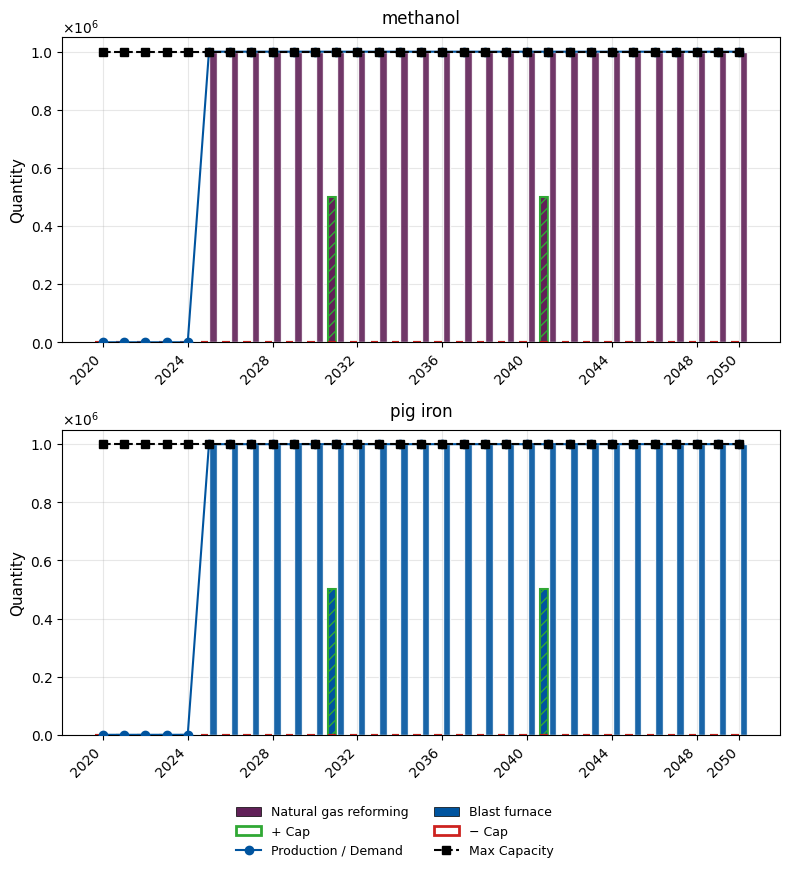
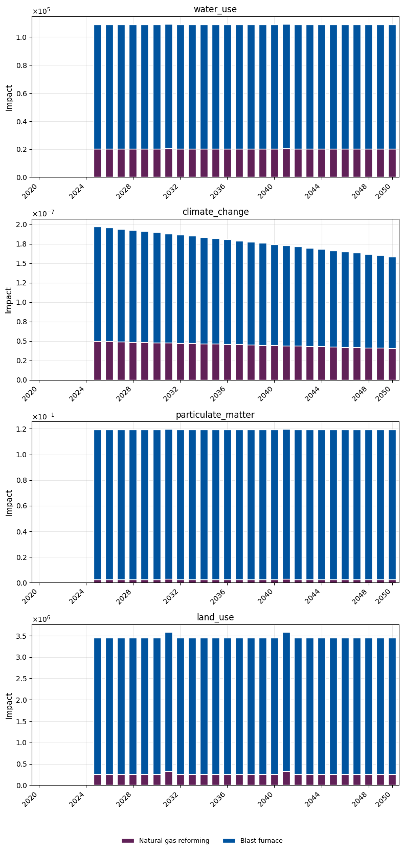
Scenario 1: Baseline
Baseline scenario: background databases are frozen at 2020 (no technological progress in the background system). This isolates the effect of foreground process choices.
# Lifetimes in TIME STEPS, i.e. the number of operating years each unit delivers
# (`operation_time_limits` is inclusive, so (0, 25) is 26 steps).
LIFETIME_BLAST_FURNACE = 26
LIFETIME_NG_REFORMING = 26

# Brownfield capacity, expressed the way plant data usually comes: annual output.
ANNUAL_EXISTING_CAPACITY = 0.5e6  # kg/year per vintage

# `existing_capacity` counts PROCESS UNITS, and one unit delivers its whole
# production temporal distribution over its entire lifetime (optimex >= 0.7.0).
# An annual capacity therefore has to be multiplied by the number of operating
# years to become a unit count. Skipping this conversion silently shrinks the
# brownfield fleet by a factor of the lifetime, and the optimizer replaces the
# missing capacity with new build.
existing_capacities = {
    ("Blast furnace", 2005): ANNUAL_EXISTING_CAPACITY * LIFETIME_BLAST_FURNACE,
    ("Blast furnace", 2015): ANNUAL_EXISTING_CAPACITY * LIFETIME_BLAST_FURNACE,
    ("Natural gas reforming", 2005): ANNUAL_EXISTING_CAPACITY * LIFETIME_NG_REFORMING,
    ("Natural gas reforming", 2015): ANNUAL_EXISTING_CAPACITY * LIFETIME_NG_REFORMING,
}

no_background_evolution_mapping = {
    ("ei312_REMIND-EU_SSP2_NDC_2020", year): 1.0 for year in range(2020, 2051)
}

optimization_model_inputs_baseline = manager.override(
    existing_capacity=existing_capacities,
    mapping=no_background_evolution_mapping,
    vintage_improvements=None,
)
from optimex import optimizer

model_baseline = optimizer.create_model(
    optimization_model_inputs_baseline,
    name="no_evolution",
    objective_category="climate_change",
)
2026-08-20 19:56:25.083 | INFO     | optimex.optimizer:create_model:138 - Creating sets
2026-08-20 19:56:25.084 | INFO     | optimex.optimizer:create_model:178 - Creating parameters
2026-08-20 19:56:25.257 | INFO     | optimex.optimizer:create_model:563 - Creating variables
m_baseline, obj_baseline, results_baseline = optimizer.solve_model(
    model_baseline, solver_name="gurobi", tee=False
)
2026-08-20 19:56:30.826 | INFO     | optimex.optimizer:solve_model:1227 - Solver [gurobi] termination: optimal
2026-08-20 19:56:30.840 | INFO     | optimex.optimizer:solve_model:1239 - Objective (scaled): 175.399
2026-08-20 19:56:30.841 | INFO     | optimex.optimizer:solve_model:1240 - Objective (real):   4.66334e-06
from optimex import postprocessing

pp_baseline = postprocessing.PostProcessor(m_baseline, plot_config={"figsize": (8, 4)})
pp_baseline.get_characterized_dynamic_inventory(
    base_lcia_method=method_climate_change
)

# Optional: export the results to disk, e.g. for external plotting or archiving.
# Not needed to run this notebook - uncomment if you want the files.

# pp_baseline.df_dynamic_inventory.to_excel(
#     "dynamic_inventory_no_evolution.xlsx"
# )
# pp_baseline.df_characterized_inventory.to_excel(
#     "characterized_inventory_no_evolution.xlsx"
# )
# pp_baseline.df_production.to_excel("production_no_evolution.xlsx")
# pp_baseline.df_demand.to_excel("demand_no_evolution.xlsx")
# pp_baseline.get_production_capacity().to_excel(
#     "capacity_no_evolution.xlsx"
# )
# pp_baseline.df_impacts.to_excel("impacts_no_evolution.xlsx")
2026-08-20 19:56:31.997 | INFO | dynamic_characterization.dynamic_characterization:characterize:82 - No custom dynamic characterization functions provided. Using default dynamic characterization functions. The flows that are characterized are based on the selection of the initially chosen impact category.
| date | amount | flow | activity | |
|---|---|---|---|---|
| 0 | 2026-01-01 05:49:12 | -2.584175e-12 | 267655084705837177 | Blast furnace |
| 1 | 2026-01-01 05:49:12 | -5.030276e-16 | 267655084332544077 | Natural gas reforming |
| 2 | 2026-01-01 05:49:12 | -1.637677e-16 | 267655084332544077 | Blast furnace |
| 3 | 2026-01-01 05:49:12 | -7.637907e-18 | 267655083766312992 | Blast furnace |
| 4 | 2026-01-01 05:49:12 | -6.490623e-19 | 267655083766312992 | Natural gas reforming |
| ... | ... | ... | ... | ... |
| 327131 | 2126-01-01 16:08:24 | 2.261536e-11 | 267655083921502208 | Blast furnace |
| 327132 | 2126-01-01 16:08:24 | 7.644926e-11 | 267655083896336466 | Natural gas reforming |
| 327133 | 2126-01-01 16:08:24 | 2.562047e-10 | 267655084475150457 | Natural gas reforming |
| 327134 | 2126-01-01 16:08:24 | 2.808755e-10 | 267655083896336466 | Blast furnace |
| 327135 | 2126-01-01 16:08:24 | 8.583475e-10 | 267655084475150457 | Blast furnace |
327136 rows × 4 columns
# Persist the baseline DESIGN (real-unit decision variables) + objective so the
# Scenario can run WITHOUT keeping m_baseline in RAM.
import json as _json
import pyomo.environ as _pyo

baseline_design = {
    "obj_baseline": float(obj_baseline),
    "installation": {
        f"{p}\t{t}": float(_pyo.value(m_baseline.var_installation[p, t]))
        for p in m_baseline.PROCESS
        for t in m_baseline.SYSTEM_TIME
    },
    "operation": {
        f"{p}\t{v}\t{t}": float(_pyo.value(m_baseline.var_operation[p, v, t]))
        for (p, v, t) in m_baseline.ACTIVE_VINTAGE_TIME
    },
}
with open("data/baseline_design.json", "w") as _f:
    _json.dump(baseline_design, _f)
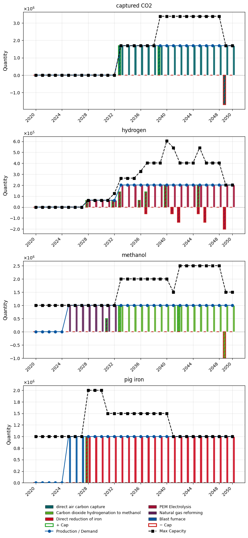
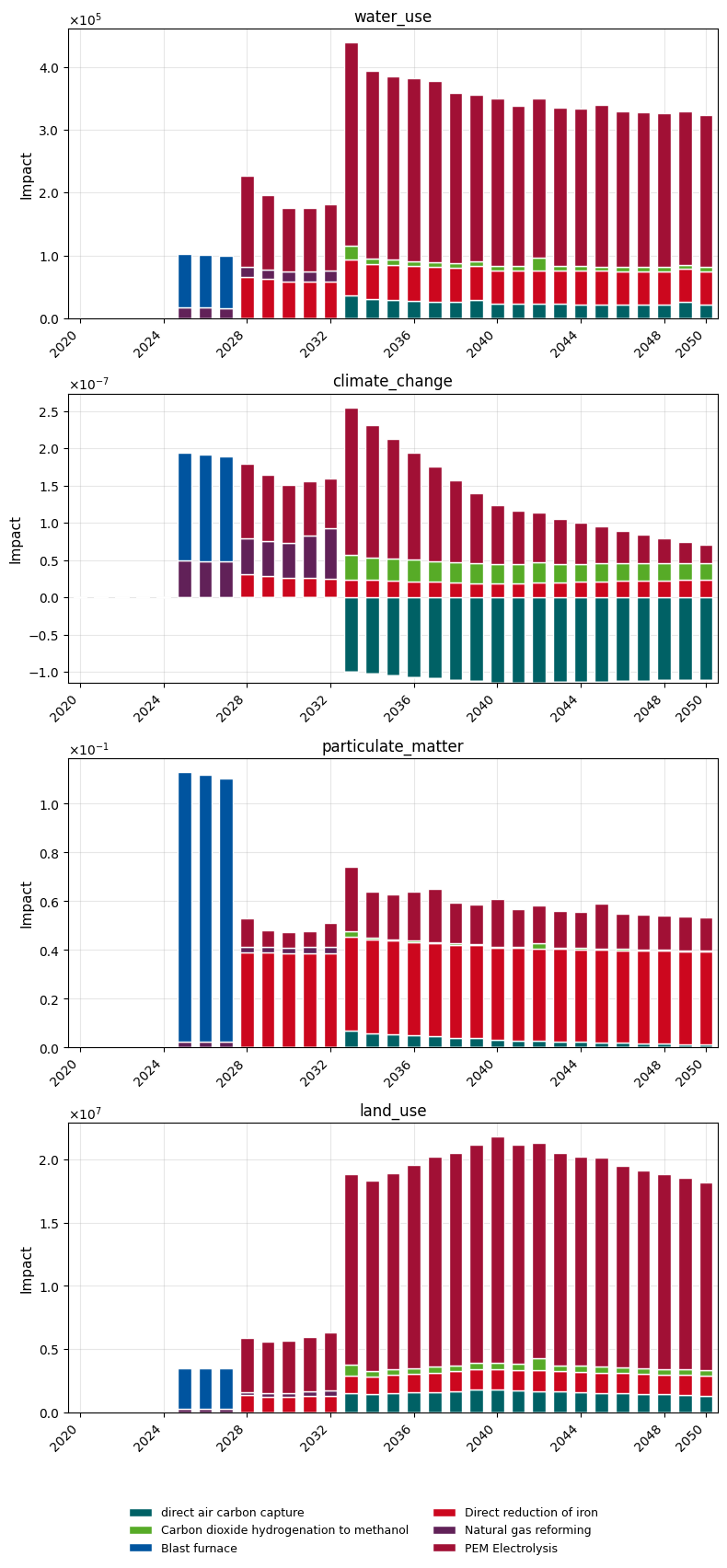
Scenario 2: Evolution
Background databases evolve according to the REMIND-EU SSP2-NDC scenario (interpolated between 2020-2100). This reflects decarbonization of electricity grids, material supply chains, etc.
manager.load_inputs("data/2026-05-28_model_inputs_2050.json")

vintage_improvements = {
    ("PEM Electrolysis", electricity_lv["code"], 2020): 1,
    ("PEM Electrolysis", electricity_lv["code"], 2030): 0.97,
    ("PEM Electrolysis", electricity_lv["code"], 2040): 0.95,
    ("PEM Electrolysis", electricity_lv["code"], 2050): 0.94,
    ("direct air carbon capture", electricity_mv["code"], 2020): 1,
    ("direct air carbon capture", electricity_mv["code"], 2030): 0.96,
    ("direct air carbon capture", electricity_mv["code"], 2040): 0.94,
    ("direct air carbon capture", electricity_mv["code"], 2050): 0.93,
    ("direct air carbon capture", heat["code"], 2020): 1,
    ("direct air carbon capture", heat["code"], 2030): 0.95,
    ("direct air carbon capture", heat["code"], 2040): 0.92,
    ("direct air carbon capture", heat["code"], 2050): 0.90,
    ("Carbon dioxide hydrogenation to methanol", co2["code"], 2020): 1,
    ("Carbon dioxide hydrogenation to methanol", co2["code"], 2030): 0.98,
    ("Carbon dioxide hydrogenation to methanol", co2["code"], 2040): 0.97,
    ("Carbon dioxide hydrogenation to methanol", co2["code"], 2050): 0.96,
    ("Carbon dioxide hydrogenation to methanol", electricity_lv["code"], 2020): 1,
    ("Carbon dioxide hydrogenation to methanol", electricity_lv["code"], 2030): 0.98,
    ("Carbon dioxide hydrogenation to methanol", electricity_lv["code"], 2040): 0.97,
    ("Carbon dioxide hydrogenation to methanol", electricity_lv["code"], 2050): 0.96,
}

optimization_model_inputs_evolution = manager.override(
    existing_capacity=existing_capacities,
    vintage_improvements=vintage_improvements,
)
from optimex import optimizer

model_evolution = optimizer.create_model(
    optimization_model_inputs_evolution,
    name="evolution",
    objective_category="climate_change",
)
2026-08-20 19:56:32.737 | INFO     | optimex.optimizer:create_model:138 - Creating sets
2026-08-20 19:56:32.738 | INFO     | optimex.optimizer:create_model:178 - Creating parameters
2026-08-20 19:56:32.920 | INFO     | optimex.optimizer:create_model:563 - Creating variables
m_evolution, obj_evolution, results_evolution = optimizer.solve_model(
    model_evolution, solver_name="gurobi", tee=False
)
2026-08-20 19:56:33.841 | INFO     | optimex.optimizer:solve_model:1227 - Solver [gurobi] termination: optimal
2026-08-20 19:56:33.853 | INFO     | optimex.optimizer:solve_model:1239 - Objective (scaled): 65.806
2026-08-20 19:56:33.854 | INFO     | optimex.optimizer:solve_model:1240 - Objective (real):   1.74958e-06
from optimex import postprocessing

pp_evolution = postprocessing.PostProcessor(m_evolution, plot_config={"figsize": (8, 4)})
# Persist evolution objective scalars for the Scenario 4 summary
# so it can run without keeping m_evolution / pp_evolution in RAM.
import json as _json

_s_evol = pp_evolution.get_impacts()["climate_change"].sum(axis=1)
evolution_results = {
    "obj_evolution": float(obj_evolution),
    "climate_per_year": {int(y): float(v) for y, v in _s_evol.items()},
}
with open("data/evolution_results.json", "w") as _f:
    _json.dump(evolution_results, _f)
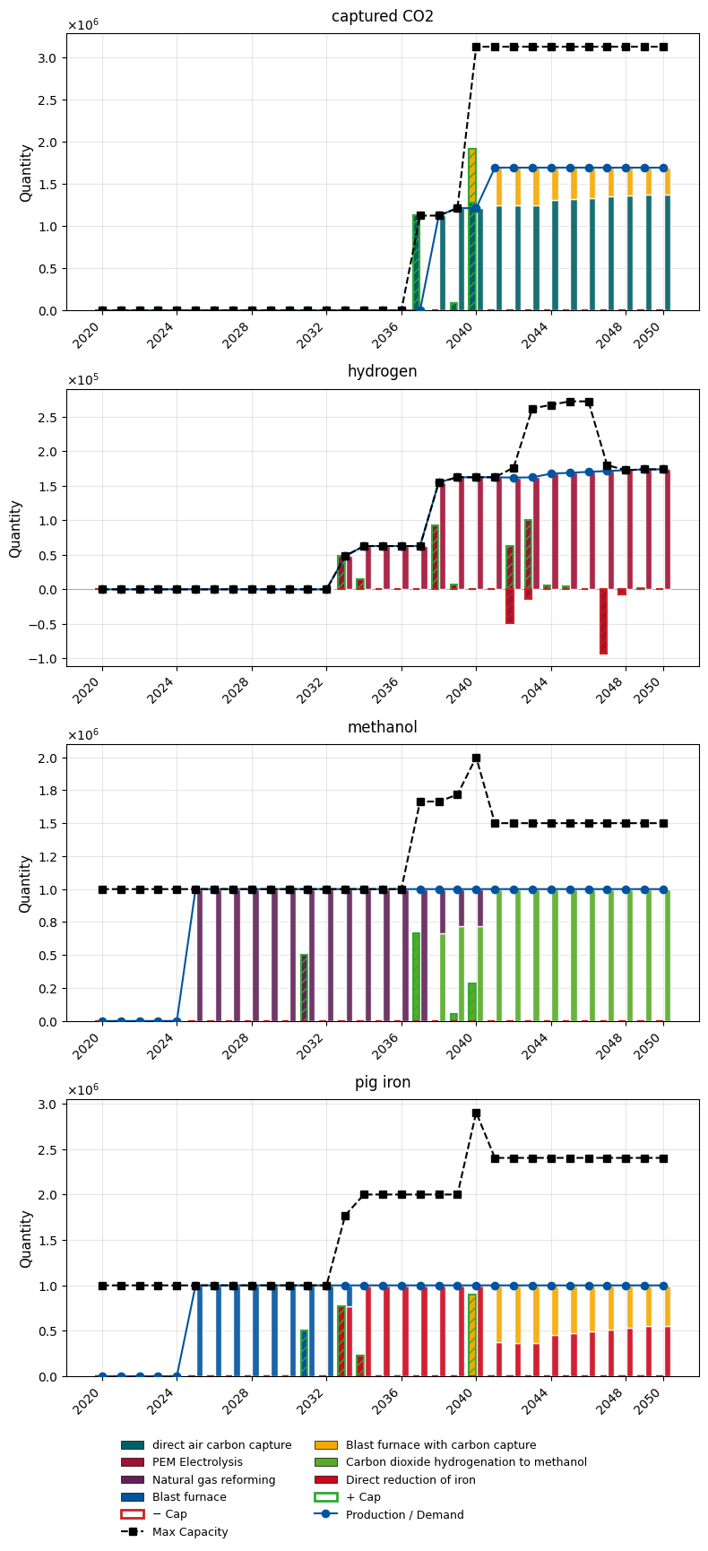
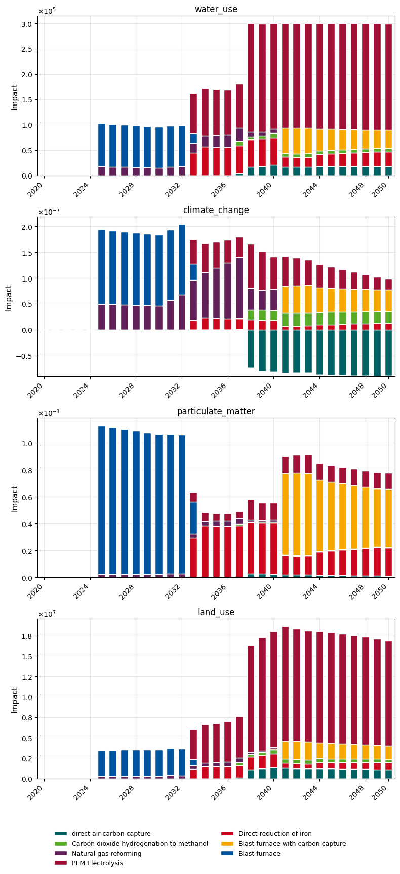
Scenario 3: Water Use and Iridium Resource constraint
Adds a maximum annual water use impact limit (300,000 units/year) and a cumulative iridium resource limit (1.125 kg) on top of the climate change objective. This demonstrates how constraints affect deployment decisions.
The iridium budget is a demonstrative one: it is set to roughly 55% of the iridium the unconstrained Scenario 2 pathway would consume, so the constraint binds without shutting the green route down entirely.
manager.load_inputs("data/2026-05-28_model_inputs_2050.json")

start_year = 2025
end_year = 2051  # range is exclusive, so this covers up to 2060
reduction_rate = 0

base_water_limit = 300_000

# Cumulative iridium budget, in kg. All iridium in this system sits in PEM stack
# construction, so this is effectively a cap on how much electrolysis can be built.
# The unconstrained evolution optimum (Scenario 2) consumes ~2.06 kg, so 1.125 kg
# caps the resource at ~55% of the unconstrained requirement: tight enough to bind,
# loose enough to still allow partial green methanol deployment.
#
# This was 0.125 kg before optimex 0.7.0. Installation impacts, and with them the
# stack material demand per kg of hydrogen, were under-counted by the length of the
# PEM operation window (9 steps), so the old budget bought ~9x more electrolysis
# than it actually pays for.
iridium_budget = 1.125

optimization_model_inputs_constrained = manager.override(
    existing_capacity=existing_capacities,
    vintage_improvements=vintage_improvements,
    category_impact_limits={
        ("water_use", year): base_water_limit
        * ((1 - reduction_rate) ** (year - start_year))
        for year in range(start_year, end_year)
    },
    cumulative_flow_limits_max={
        iridium["code"]: iridium_budget,
    },
)
from optimex import optimizer

model_constrained = optimizer.create_model(
    optimization_model_inputs_constrained,
    name="constrained",
    objective_category="climate_change",
)
2026-08-20 19:56:35.121 | INFO     | optimex.optimizer:create_model:138 - Creating sets
2026-08-20 19:56:35.121 | INFO     | optimex.optimizer:create_model:178 - Creating parameters
2026-08-20 19:56:35.298 | INFO     | optimex.optimizer:create_model:563 - Creating variables
m_constrained, obj_constrained, results_constrained = optimizer.solve_model(
    model_constrained, solver_name="gurobi", tee=False
)  # any accurate LP solver works here: "gurobi", "cplex", "highs" (not "glpk", see above)
2026-08-20 19:56:36.024 | INFO     | optimex.optimizer:solve_model:1227 - Solver [gurobi] termination: optimal
2026-08-20 19:56:36.037 | INFO     | optimex.optimizer:solve_model:1239 - Objective (scaled): 85.2735
2026-08-20 19:56:36.037 | INFO     | optimex.optimizer:solve_model:1240 - Objective (real):   2.26716e-06
from optimex import postprocessing

pp_constrained = postprocessing.PostProcessor(m_constrained, plot_config={"figsize": (8, 4)})
pp_constrained.get_characterized_dynamic_inventory(
    base_lcia_method=method_climate_change
)

# Optional: export the results to disk, e.g. for external plotting or archiving.
# Not needed to run this notebook - uncomment if you want the files.

# pp_constrained.df_dynamic_inventory.to_excel(
#     "dynamic_inventory_constrained.xlsx"
# )
# pp_constrained.df_characterized_inventory.to_excel(
#     "characterized_inventory_constrained.xlsx"
# )
# pp_constrained.df_production.to_excel("production_constrained.xlsx")
# pp_constrained.df_demand.to_excel("demand_constrained.xlsx")
# pp_constrained.get_production_capacity().to_excel(
#     "capacity_constrained.xlsx"
# )
# pp_constrained.df_impacts.to_excel("impacts_constrained.xlsx")
2026-08-20 19:56:37.453 | INFO | dynamic_characterization.dynamic_characterization:characterize:82 - No custom dynamic characterization functions provided. Using default dynamic characterization functions. The flows that are characterized are based on the selection of the initially chosen impact category.
| date | amount | flow | activity | |
|---|---|---|---|---|
| 0 | 2020-12-31 05:49:12 | -2.721806e-18 | 267655084332544077 | Natural gas reforming |
| 1 | 2020-12-31 05:49:12 | -9.746723e-20 | 267655083766312992 | Natural gas reforming |
| 2 | 2020-12-31 05:49:12 | 1.303085e-43 | 267655084806500426 | Natural gas reforming |
| 3 | 2020-12-31 05:49:12 | 1.637343e-42 | 267655084563230730 | Natural gas reforming |
| 4 | 2020-12-31 05:49:12 | 3.554478e-26 | 267655084705837111 | Natural gas reforming |
| ... | ... | ... | ... | ... |
| 628944 | 2126-01-01 16:08:24 | 5.883176e-11 | 267655084475150457 | Direct reduction of iron |
| 628945 | 2126-01-01 16:08:24 | 6.061699e-11 | 267655084475150457 | Natural gas reforming |
| 628946 | 2126-01-01 16:08:24 | 6.585316e-11 | 267655084705837139 | PEM Electrolysis |
| 628947 | 2126-01-01 16:08:24 | 7.042168e-11 | 267655083959250953 | PEM Electrolysis |
| 628948 | 2126-01-01 16:08:24 | 1.771054e-10 | 267655084475150457 | Carbon dioxide hydrogenation to methanol |
628949 rows × 4 columns
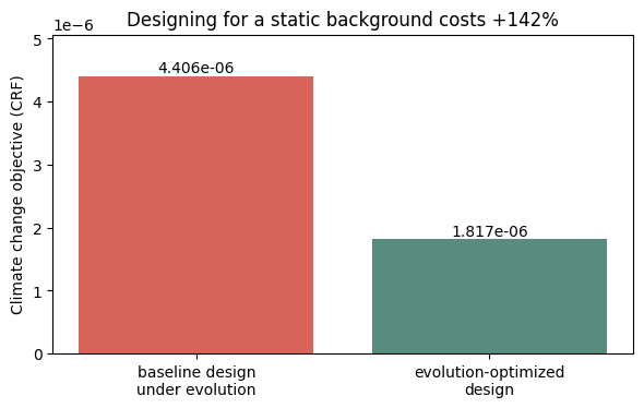
Scenario 4: Baseline Design Under Evolution
How much worse is a portfolio optimized for a static background once the world actually evolves? We take the optimal design from Scenario 1 (baseline / no evolution — installation and operation decided under a frozen 2020 background) and evaluate its climate impact under the Scenario 2 evolution conditions (evolving REMIND-EU SSP2-NDC background + vintage improvements).
The design is fully fixed: every var_installation and var_operation is locked to the baseline optimum, so there are no degrees of freedom left and no re-optimization is needed — we rebuild the evolution-structured model and simply evaluate its objective expression. var_installation and var_operation are already in real units (see PostProcessor), so the variables need no rescaling; only the objective is denormalized (scaled_obj * fg_scale * cat_scale), exactly as solve_model does.
Comparing this fixed baseline design against the freely-optimized evolution design (Scenario 2) — both under the same evolution conditions — quantifies the penalty of having designed for the wrong background.
import json
import pyomo.environ as pyo
from optimex import optimizer

# Load the baseline design from disk (no need for m_baseline in RAM).
with open("data/baseline_design.json") as f:
    baseline_design = json.load(f)
obj_baseline = baseline_design["obj_baseline"]

# Rebuild the evolution-structured model (same as Scenario 2). This is the ONLY
# optimization model that needs to be in RAM for Scenario 4.
manager.load_inputs("data/2026-05-28_model_inputs_2050.json")
optimization_model_inputs_fixed = manager.override(
    existing_capacity=existing_capacities,
    vintage_improvements=vintage_improvements,
)
model_fixed = optimizer.create_model(
    optimization_model_inputs_fixed,
    name="baseline_design_under_evolution",
    objective_category="climate_change",
)

# Fixing the design to the baseline values (already in real units, see PostProcessor).
for p in model_fixed.PROCESS:
    for t in model_fixed.SYSTEM_TIME:
        model_fixed.var_installation[p, t].fix(baseline_design["installation"][f"{p}\t{t}"])
for (p, v, t) in model_fixed.ACTIVE_VINTAGE_TIME:
    model_fixed.var_operation[p, v, t].fix(baseline_design["operation"][f"{p}\t{v}\t{t}"])

# Denormalize the objective exactly as solve_model does: scaled_obj * fg_scale * cat_scale
scaled_obj = pyo.value(model_fixed.OBJ)
fg_scale = model_fixed.scales["foreground"]
cat_scale = model_fixed.scales["characterization"]["climate_change"]
obj_fixed = scaled_obj * fg_scale * cat_scale
2026-08-20 19:56:38.729 | INFO     | optimex.optimizer:create_model:138 - Creating sets
2026-08-20 19:56:38.730 | INFO     | optimex.optimizer:create_model:178 - Creating parameters
2026-08-20 19:56:38.908 | INFO     | optimex.optimizer:create_model:563 - Creating variables


WARNING (W1001): Setting Var 'var_operation[Natural gas reforming,2021,2028]'
to a value `-3.167332229825348e-11` (float) not in domain NonNegativeReals.
    See also https://pyomo.readthedocs.io/en/stable/errors.html#w1001
WARNING (W1001): Setting Var 'var_operation[Natural gas reforming,2022,2025]'
to a value `-3.167332229825348e-11` (float) not in domain NonNegativeReals.
    See also https://pyomo.readthedocs.io/en/stable/errors.html#w1001
WARNING (W1001): Setting Var 'var_operation[Natural gas reforming,2023,2030]'
to a value `-3.167332229825348e-11` (float) not in domain NonNegativeReals.
    See also https://pyomo.readthedocs.io/en/stable/errors.html#w1001
WARNING (W1001): Setting Var 'var_operation[Natural gas reforming,2024,2026]'
to a value `-3.167332229825348e-11` (float) not in domain NonNegativeReals.
    See also https://pyomo.readthedocs.io/en/stable/errors.html#w1001
WARNING (W1001): Setting Var 'var_operation[Natural gas reforming,2025,2027]'
to a value `-3.167332229825348e-11` (float) not in domain NonNegativeReals.
    See also https://pyomo.readthedocs.io/en/stable/errors.html#w1001
WARNING (W1001): Setting Var 'var_operation[Natural gas reforming,2026,2029]'
to a value `-3.167332229825348e-11` (float) not in domain NonNegativeReals.
    See also https://pyomo.readthedocs.io/en/stable/errors.html#w1001
WARNING (W1001): Setting Var 'var_operation[Natural gas reforming,2039,2042]'
to a value `-6.334664459650696e-11` (float) not in domain NonNegativeReals.
    See also https://pyomo.readthedocs.io/en/stable/errors.html#w1001
WARNING (W1001): Setting Var 'var_operation[Natural gas reforming,2040,2043]'
to a value `-6.334664459650696e-11` (float) not in domain NonNegativeReals.
    See also https://pyomo.readthedocs.io/en/stable/errors.html#w1001
WARNING (W1001): Setting Var 'var_operation[Natural gas reforming,2040,2050]'
to a value `-6.334664459650696e-11` (float) not in domain NonNegativeReals.
    See also https://pyomo.readthedocs.io/en/stable/errors.html#w1001
WARNING (W1001): Setting Var 'var_operation[Natural gas reforming,2041,2044]'
to a value `-6.334664459650696e-11` (float) not in domain NonNegativeReals.
    See also https://pyomo.readthedocs.io/en/stable/errors.html#w1001
WARNING (W1001): Setting Var 'var_operation[Natural gas reforming,2041,2046]'
to a value `-6.334664459650696e-11` (float) not in domain NonNegativeReals.
    See also https://pyomo.readthedocs.io/en/stable/errors.html#w1001
WARNING (W1001): Setting Var 'var_operation[Natural gas reforming,2042,2045]'
to a value `-6.334664459650696e-11` (float) not in domain NonNegativeReals.
    See also https://pyomo.readthedocs.io/en/stable/errors.html#w1001
WARNING (W1001): Setting Var 'var_operation[Natural gas reforming,2043,2047]'
to a value `-6.334664459650696e-11` (float) not in domain NonNegativeReals.
    See also https://pyomo.readthedocs.io/en/stable/errors.html#w1001
WARNING (W1001): Setting Var 'var_operation[Natural gas reforming,2044,2048]'
to a value `-6.334664459650696e-11` (float) not in domain NonNegativeReals.
    See also https://pyomo.readthedocs.io/en/stable/errors.html#w1001
WARNING (W1001): Setting Var 'var_operation[Natural gas reforming,2046,2049]'
to a value `-6.334664459650696e-11` (float) not in domain NonNegativeReals.
    See also https://pyomo.readthedocs.io/en/stable/errors.html#w1001
WARNING (W1001): Setting Var 'var_operation[Natural gas reforming,2015,2031]'
to a value `-6.334664459650696e-11` (float) not in domain NonNegativeReals.
    See also https://pyomo.readthedocs.io/en/stable/errors.html#w1001
WARNING (W1001): Setting Var 'var_operation[Natural gas reforming,2015,2032]'
to a value `-6.334664459650696e-11` (float) not in domain NonNegativeReals.
    See also https://pyomo.readthedocs.io/en/stable/errors.html#w1001
WARNING (W1001): Setting Var 'var_operation[Natural gas reforming,2015,2033]'
to a value `-6.334664459650696e-11` (float) not in domain NonNegativeReals.
    See also https://pyomo.readthedocs.io/en/stable/errors.html#w1001
WARNING (W1001): Setting Var 'var_operation[Natural gas reforming,2015,2034]'
to a value `-6.334664459650696e-11` (float) not in domain NonNegativeReals.
    See also https://pyomo.readthedocs.io/en/stable/errors.html#w1001
WARNING (W1001): Setting Var 'var_operation[Natural gas reforming,2015,2037]'
to a value `-6.334664459650696e-11` (float) not in domain NonNegativeReals.
    See also https://pyomo.readthedocs.io/en/stable/errors.html#w1001
WARNING (W1001): Setting Var 'var_operation[Natural gas reforming,2015,2039]'
to a value `-6.334664459650696e-11` (float) not in domain NonNegativeReals.
    See also https://pyomo.readthedocs.io/en/stable/errors.html#w1001
WARNING (W1001): Setting Var 'var_operation[Blast furnace,2028,2028]' to a
value `-3.167332229825348e-11` (float) not in domain NonNegativeReals.
    See also https://pyomo.readthedocs.io/en/stable/errors.html#w1001
WARNING (W1001): Setting Var 'var_operation[Blast furnace,2040,2042]' to a
value `-6.334664459650696e-11` (float) not in domain NonNegativeReals.
    See also https://pyomo.readthedocs.io/en/stable/errors.html#w1001
WARNING (W1001): Setting Var 'var_operation[Blast furnace,2040,2043]' to a
value `-6.334664459650696e-11` (float) not in domain NonNegativeReals.
    See also https://pyomo.readthedocs.io/en/stable/errors.html#w1001
WARNING (W1001): Setting Var 'var_operation[Blast furnace,2040,2044]' to a
value `-6.334664459650696e-11` (float) not in domain NonNegativeReals.
    See also https://pyomo.readthedocs.io/en/stable/errors.html#w1001
WARNING (W1001): Setting Var 'var_operation[Blast furnace,2041,2045]' to a
value `-6.334664459650696e-11` (float) not in domain NonNegativeReals.
    See also https://pyomo.readthedocs.io/en/stable/errors.html#w1001
WARNING (W1001): Setting Var 'var_operation[Blast furnace,2042,2046]' to a
value `-6.334664459650696e-11` (float) not in domain NonNegativeReals.
    See also https://pyomo.readthedocs.io/en/stable/errors.html#w1001
WARNING (W1001): Setting Var 'var_operation[Blast furnace,2042,2047]' to a
value `-6.334664459650696e-11` (float) not in domain NonNegativeReals.
    See also https://pyomo.readthedocs.io/en/stable/errors.html#w1001
WARNING (W1001): Setting Var 'var_operation[Blast furnace,2043,2048]' to a
value `-6.334664459650696e-11` (float) not in domain NonNegativeReals.
    See also https://pyomo.readthedocs.io/en/stable/errors.html#w1001
WARNING (W1001): Setting Var 'var_operation[Blast furnace,2044,2049]' to a
value `-6.334664459650696e-11` (float) not in domain NonNegativeReals.
    See also https://pyomo.readthedocs.io/en/stable/errors.html#w1001
WARNING (W1001): Setting Var 'var_operation[Blast furnace,2015,2031]' to a
value `-6.334664459650696e-11` (float) not in domain NonNegativeReals.
    See also https://pyomo.readthedocs.io/en/stable/errors.html#w1001
WARNING (W1001): Setting Var 'var_operation[Blast furnace,2015,2032]' to a
value `-6.334664459650696e-11` (float) not in domain NonNegativeReals.
    See also https://pyomo.readthedocs.io/en/stable/errors.html#w1001
from optimex import postprocessing

pp_fixed = postprocessing.PostProcessor(model_fixed, plot_config={"figsize": (8, 4)})

# Load evolution results from disk (no need for m_evolution / pp_evolution in RAM).
with open("data/evolution_results.json") as f:
    evolution_results = json.load(f)
obj_evolution = evolution_results["obj_evolution"]

print(f"Baseline design @ baseline background (Scenario 1): {obj_baseline:.6g}")
print(f"Baseline design @ evolution background (fixed):     {obj_fixed:.6g}")
print(f"Evolution-optimized design (Scenario 2):            {obj_evolution:.6g}")
Baseline design @ baseline background (Scenario 1): 4.66334e-06
Baseline design @ evolution background (fixed):     4.41788e-06
Evolution-optimized design (Scenario 2):            1.74958e-06
import pandas as pd

abs_gap = obj_fixed - obj_evolution
rel_gap = abs_gap / obj_evolution

summary = pd.DataFrame(
    {
        "objective (climate_change)": [obj_baseline, obj_fixed, obj_evolution],
        "background": ["frozen 2020", "evolution", "evolution"],
        "design": ["baseline-optimized", "baseline-optimized", "evolution-optimized"],
    },
    index=["baseline", "baseline_design_under_evolution", "evolution_optimum"],
)
print(summary.to_string())
print(
    f"\nUnder evolution conditions, the baseline design causes +{rel_gap * 100:.1f}% "
    f"climate impact vs the evolution-optimized design (absolute: {abs_gap:.4e})."
)
# Optional: summary.to_excel("comparison_baseline_design_under_evolution.xlsx")
                                 objective (climate_change)   background               design
baseline                                           0.000005  frozen 2020   baseline-optimized
baseline_design_under_evolution                    0.000004    evolution   baseline-optimized
evolution_optimum                                  0.000002    evolution  evolution-optimized

Under evolution conditions, the baseline design causes +152.5% climate impact vs the evolution-optimized design (absolute: 2.6683e-06).
import matplotlib.pyplot as plt

fig, ax = plt.subplots(figsize=(6, 4))
labels = ["baseline design\nunder evolution", "evolution-optimized\ndesign"]
values = [obj_fixed, obj_evolution]
bars = ax.bar(labels, values, color=["#d96459", "#588c7e"])
ax.set_ylabel("Climate change objective (CRF)")
ax.set_title(f"Designing for a static background costs +{rel_gap * 100:.0f}%")
for b, val in zip(bars, values):
    ax.text(b.get_x() + b.get_width() / 2, val, f"{val:.3e}", ha="center", va="bottom")
ax.margins(y=0.15)
plt.tight_layout()
plt.show()
imp_fixed = pp_fixed.get_impacts()
# Optional: pp_fixed.df_impacts.to_excel("impacts_baseline_under_evolution.xlsx")

# Quick preview: annual RF (CRF per emission-year).
s_ref = pp_baseline.get_impacts()["climate_change"].sum(axis=1)   # baseline design, baseline background
s_fixed = imp_fixed["climate_change"].sum(axis=1)                 # baseline design, evolution background
s_evol = pd.Series(
    {int(y): v for y, v in evolution_results["climate_per_year"].items()}
).sort_index()                                                    # evolution-optimized

fig, ax = plt.subplots(figsize=(8, 4))
ax.fill_between(s_fixed.index, s_evol.reindex(s_fixed.index).values, s_fixed.values,
                where=(s_fixed.values >= s_evol.reindex(s_fixed.index).values),
                color="#CC071E", alpha=0.15, label="excess impact")
ax.plot(s_ref.index, s_ref.values, color="#646567", linestyle="--",
        label="baseline design, baseline background")
ax.plot(s_fixed.index, s_fixed.values, color="#CC071E",
        label="baseline design, evolution background")
ax.plot(s_evol.index, s_evol.values, color="#57AB27", label="evolution-optimized")
ax.set_xlabel("Year"); ax.set_ylabel("Annual RF (CRF per emission-year)")
ax.legend(); ax.grid(alpha=0.3)
plt.tight_layout(); plt.show()
